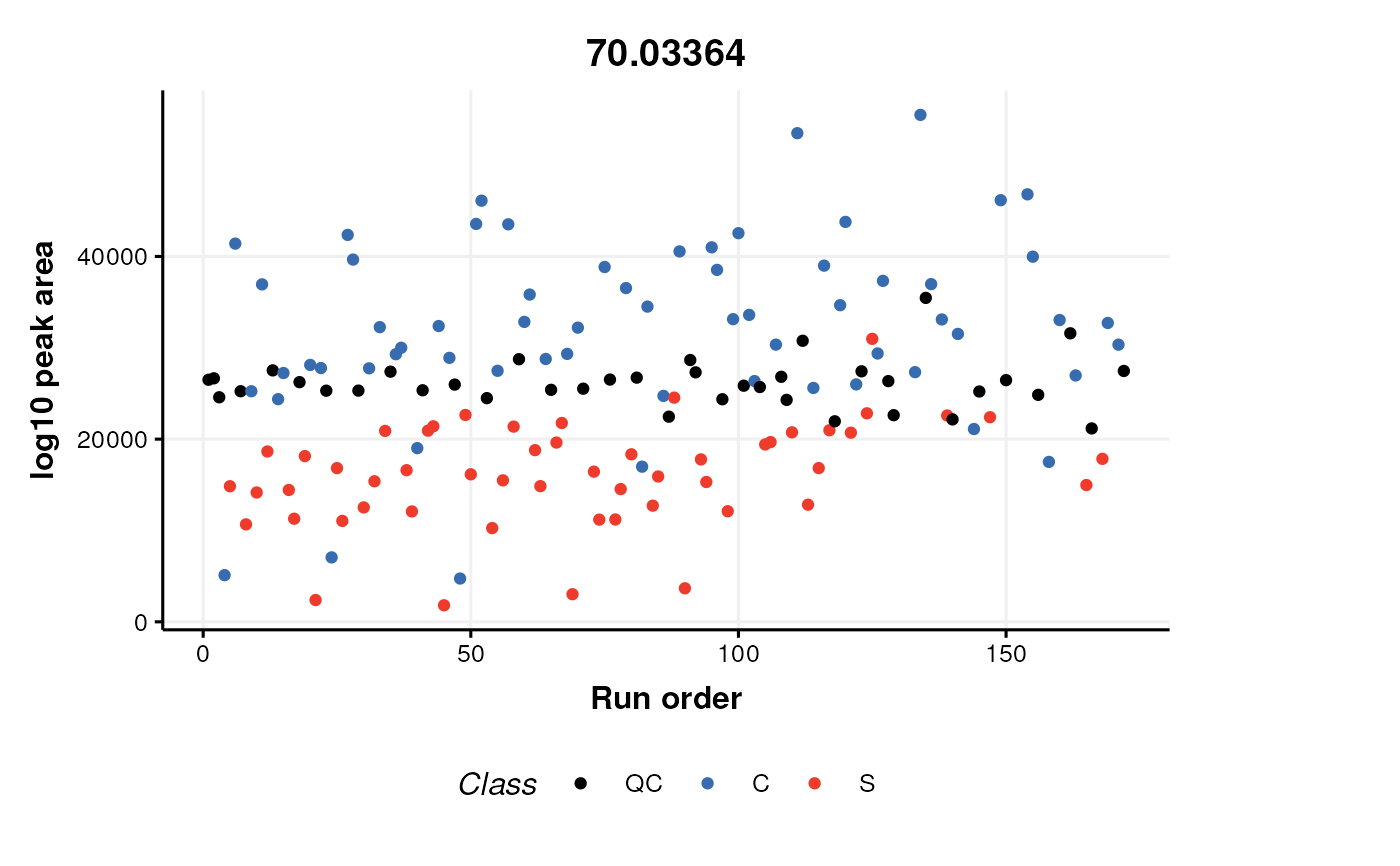
A plot visualising the change in intensity of a feature with a continuous variable such as time, dose, or run order.
Usage
feature_profile(
  run_order,
  qc_label,
  qc_column,
  colour_by,
  feature_to_plot,
  plot_sd = FALSE,
  ...
)
Arguments
- run_order
(character) The sample-meta column name containing run order.
- qc_label
(character) The label used to identify QC samples.
- qc_column
(character) The sample-meta column name containing the labels used to identify QC samples.
- colour_by
(character) The sample-meta column name to used to colour the plot.
- feature_to_plot
(numeric, character, integer) The name or column id of the plotted feature.
- plot_sd
(logical) Plot standard deviation. Allowed values are limited to the following:
"TRUE": Standard deviation of samples and QCs are included on the plot."FALSE": Standard deviation is not plotted.
The default is
FALSE.- ...
Additional slots and values passed to
struct_class.
Value
A
feature_profile
object. This object has no output slots.
See chart_plot in the struct package to plot this chart object.
Inheritance
A feature_profile object inherits the following struct classes: [feature_profile] >> [chart] >> [struct_class]
Examples
M = feature_profile(
      run_order = character(0),
      qc_label = character(0),
      qc_column = character(0),
      colour_by = character(0),
      feature_to_plot = numeric(0),
      plot_sd = FALSE)

D = MTBLS79_DatasetExperiment()
C = feature_profile(run_order='run_order',
    qc_label='QC',
    qc_column='Class',
    colour_by='Class',
    feature_to_plot=1)
chart_plot(C,D)
#> Warning: Removed 18 rows containing missing values or values outside the scale range
#> (`geom_point()`).
