Annotation of mixtures of standards
Gavin Rhys Lloyd
2024-11-05
Source:vignettes/annotate_mixtures.Rmd
annotate_mixtures.RmdGetting Started
The latest versions of struct and
MetMashR that are compatible with your current R version
can be installed using BiocManager.
# install BiocManager if not present
if (!requireNamespace("BiocManager", quietly = TRUE)) {
    install.packages("BiocManager")
}

# install MetMashR and dependencies
BiocManager::install("MetMashR")
Once installed you can activate the packages in the usual way:
Introduction
Mixtures of standards can be used to build annotation libraries. In LCMS these libraries can be collected using the same chromatography and instrument as the samples. Such a library allows high-confidence (MSI level 1) detection/annotation of MTox metabolites, in comparison to external databases/sources that rely on m/z only or in-silico predictions.
In this vignette we will explore the annotations generated using Compound Discoverer (CD) and LipidSearch (LS) for several mixtures of standards.
As the content of the standard mixtures is known, we can assess the ability of CD and LS to annotate these metabolites.
Input data
The data collected corresponds to mixtures of high-purity standards measured using LCMS, with the intention of building an internally measured library including m/z and retention times for each standard.
Analysis of the standard mixtures resulted in four data tables: HILIC_NEG, HILIC_POS, LIPIDS_POS and LIPIDS_NEG. We will loosely refer to these as “assays”.
All four assays were used as input to both Compound Discoverer (CD) and LipidSearch (LS) software, which are software tools commonly used to annotation LCMS datasets.
Importing the annotations
MetMashR includes cd_source and
ls_source objects. These objects read the output files from
CD and LS and parse them into an annotation_table
object.
Importing the annotation tables isn’t always enough; sometimes they
need to be cleaned or processed further. We therefore define two
MetMashR workflows, one for CD and one for LS, in which we
import the tables and then apply source-specific cleaning.
Importing Compound Discoverer annotations
The CD file format expected by cd_source is Excel
format; see [TODO] for details on how to generate this format from
CD.
For the CD MetMashR workflow we would like to:
- Import CD annotations and convert to
annotation_tableformat - Filter to only include “Full match” annotations
- Resolve duplicates
When we import the annotations, we add a column indicating which
assay the annotations are associated with, include a tag
for each row indicating both the source and the assay. This will be
useful later when processing the combined tables.
The resolution of duplicates is needed because CD might assign the
same metabolite + adduct to multiple peaks. Here we choose the match
with highest mzcloud score using the select_max helper
function with the combine_records` object. This object is a wrapper for
[dplyr::reframe()].
# prepare workflow
M <- import_source() +
    add_labels(
        labels = c(
            assay = "placeholder", # will be replaced later
            source_name = "CD"
        )
    ) +
    filter_labels(
        column_name = "compound_match",
        labels = "Full match",
        mode = "include"
    ) +
    filter_labels(
        column_name = "compound_match",
        labels = "Full match",
        mode = "include"
    ) +
    filter_range(
        column_name = "library_ppm_diff",
        upper_limit = 2,
        lower_limit = -2,
        equal_to = FALSE
    ) +
    combine_records(
        group_by = c("compound", "ion"),
        default_fcn = select_max(
            max_col = "mzcloud_score",
            keep_NA = FALSE,
            use_abs = TRUE
        )
    )

# place to store results
CD <- list()
for (assay in c("HILIC_NEG", "HILIC_POS", "LIPIDS_NEG", "LIPIDS_POS")) {
    # prepare source
    AT <- cd_source(
        source = c(
            system.file(
                paste0("extdata/MTox/CD/", assay, ".xlsx"),
                package = "MetMashR"
            ),
            system.file(
                paste0("extdata/MTox/CD/", assay, "_comp.xlsx"),
                package = "MetMashR"
            )
        ),
        tag = paste0("CD_", assay)
    )

    # update labels in workflow
    M[2]$labels$assay <- assay

    # apply workflow to source
    CD[[assay]] <- model_apply(M, AT)
}
The CD variable is now a list containing the workflow
for each assay.
The default output of each workflow is a processed
lcms_table, which is an extension of
annotation_table that requires both an m/z and a retention
time column to be defined.
A summary of the table for e.g. the HILIC_NEG assay can be displayed on the console:
predicted(CD$HILIC_NEG)
#> A "cd_source" object
#> --------------------
#> name:          LCMS table
#> description:   An LCMS table extends [`annotation_table()`] to represent annotation data for an LCMS
#>                  experiment. Columns representing m/z and retention time are required for an
#>                  `lcms_table`.
#> input params:  sheets
#> annotations:   219 rows x 21 columns
The HILIC_NEG table is shown below.
MetMashR workflows store the output after each step. We
can use this to explore the impact of different workflow steps. For
example, we can display the different compound matched present before
and after filtering as pie charts.
First, we create the pie chart object and specify some parameters.
C <- annotation_pie_chart(
    factor_name = "compound_match",
    label_rotation = FALSE,
    label_location = "outside",
    legend = TRUE,
    label_type = "percent",
    centre_radius = 0.5,
    centre_label = ".total"
)
Now we create the plots using chart_plot and add some
additional settings using ggplot2, and arrange the plots
using cowplot.
Note that we use square brackets to index the step of the workflow we
want to access e.g. HILIC_NEG[3].
# plot individual charts
g1 <- chart_plot(C, predicted(CD$HILIC_NEG[3])) +
    ggtitle("Compound matches\nafter filtering") +
    theme(plot.title = element_text(hjust = 0.5))


g2 <- chart_plot(C, predicted(CD$HILIC_NEG[2])) +
    ggtitle("Compound matches\nbefore filtering") +
    theme(plot.title = element_text(hjust = 0.5))


# get legend
leg <- cowplot::get_legend(g2)
#> Warning in get_plot_component(plot, "guide-box"): Multiple components found;
#> returning the first one. To return all, use `return_all = TRUE`.

# layout
cowplot::plot_grid(
    g2 + theme(legend.position = "none"),
    g1 + theme(legend.position = "none"),
    leg,
    nrow = 1,
    rel_widths = c(1, 1, 0.5)
)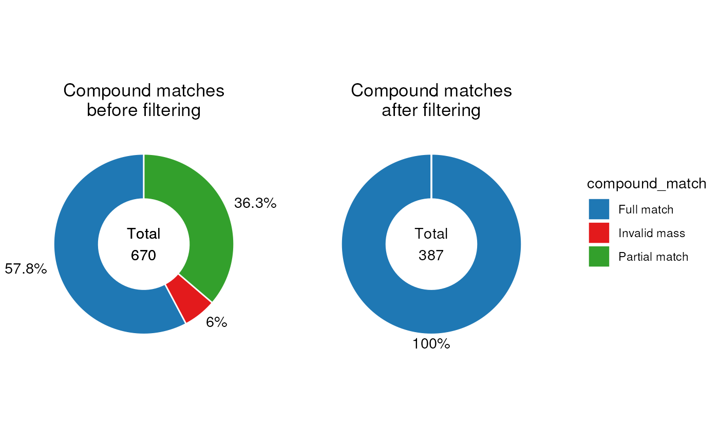
It is clear from these plots that the filter has removed all annotations without a “full match”.
We can assess the quality of the annotations be examining the histogram of ppm errors between the MS2 peaks and the library.
If there is a wide distribution then this may indicate false positives. If the distribution is offset from zero then this indicates some m/z drift is present.
C <- annotation_histogram(
    factor_name = "library_ppm_diff", vline = c(-2, 2)
)
G <- list()
G$HILIC_NEG <- chart_plot(C, predicted(CD$HILIC_NEG[2]))
G$HILIC_POS <- chart_plot(C, predicted(CD$HILIC_POS[3]))

cowplot::plot_grid(plotlist = G, labels = c("HILIC_NEG", "HILIC_POS"))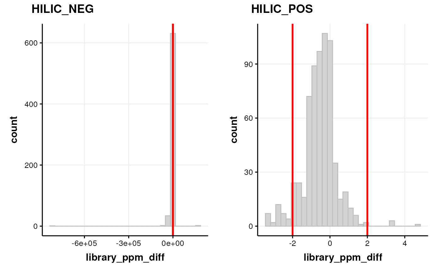
Note that we plotted the distribution based on the step before filtering by range, and set the vertical red lines equal to the range filter so that we can see which parts of the histogram are affected by the range filter.
Importing LipidSearch annotations
The file format expected by ls_source is a
.csv file. See [TODO] for details on how to generate this
format from LS.
For the MetMashR workflow we would like to:
- Import the LS annotations and convert to
annotation_tableformat - Filter the annotations to only include grades A and B
- Resolve duplicates
When we import the annotations, we add a column indicating which
assay and source the annotations are associated with. We also include a
tag for the table. This will be useful later when
processing the combined tables.
For LS we resolve duplicates by selecting the annotation with the
smallest ppm error. We use the combine_records object with
the select_min helper function to do this.
# prepare workflow
M <- import_source() +
    add_labels(
        labels = c(
            assay = "placeholder", # will be replaced later
            source_name = "LS"
        )
    ) +
    filter_labels(
        column_name = "Grade",
        labels = c("A", "B"),
        mode = "include"
    ) +
    filter_labels(
        column_name = "Grade",
        labels = c("A", "B"),
        mode = "include"
    ) +
    combine_records(
        group_by = c("LipidIon"),
        default_fcn = select_min(
            min_col = "library_ppm_diff",
            keep_NA = FALSE,
            use_abs = TRUE
        )
    )

# place to store results
LS <- list()
for (assay in c("HILIC_NEG", "HILIC_POS", "LIPIDS_NEG", "LIPIDS_POS")) {
    # prepare source
    AT <- ls_source(
        source = system.file(
            paste0("extdata/MTox/LS/MTox_2023_", assay, ".txt"),
            package = "MetMashR"
        ),
        tag = paste0("LS_", assay)
    )

    # update labels in workflow
    M[2]$labels$assay <- assay

    # apply workflow to source
    LS[[assay]] <- model_apply(M, AT)
}
The LS variable is now a list containing the workflow
for each assay.
A summary of the table for e.g. the LIPIDS_NEG assay can be displayed on the console:
predicted(LS$LIPIDS_NEG)
#> A "ls_source" object
#> --------------------
#> name:          LCMS table
#> description:   An LCMS table extends [`annotation_table()`] to represent annotation data for an LCMS
#>                  experiment. Columns representing m/z and retention time are required for an
#>                  `lcms_table`.
#> input params:  mz_column, rt_column
#> annotations:   16 rows x 14 columns
The LIPIDS_NEG table is shown below.
MetMashR workflows store the output after each step. We
can use this to explore the impact of different workflow steps. For
example, we can display the different Grades present before and after
filtering as pie charts.
C <- annotation_pie_chart(
    factor_name = "Grade",
    label_rotation = FALSE,
    label_location = "outside",
    label_type = "percent",
    legend = FALSE,
    centre_radius = 0.5,
    centre_label = ".total"
)
g1 <- chart_plot(C, predicted(LS$LIPIDS_NEG)) +
    ggtitle("Grades after filtering") +
    theme(plot.margin = unit(c(1, 1.5, 1, 1.5), "cm"))

g2 <- chart_plot(C, predicted(LS$LIPIDS_NEG[1])) +
    ggtitle("Grades before filtering") +
    theme(plot.margin = unit(c(1, 1.5, 1, 1.5), "cm"))


cowplot::plot_grid(g2, g1, nrow = 1, align = "v")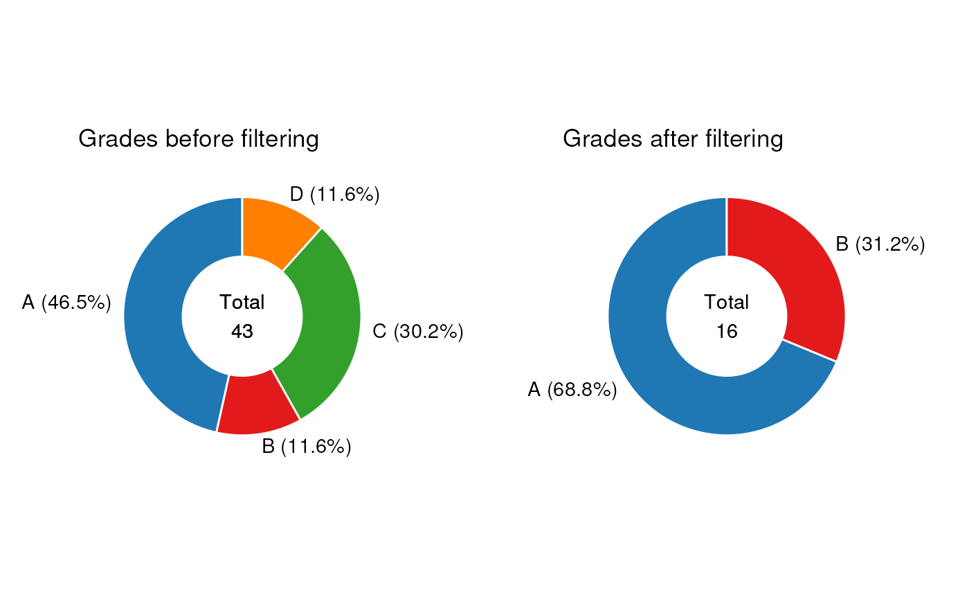
Exploratory analysis of annotation sources
The annotations imported from each source are interesting to explore graphically “within source”. We will draw a comparison “between sources” later.
In this example we generate Venn diagrams by providing several
annotation_table inputs to the chart_plot
function for an annotation_venn_chart. This allows us to
compare columns of e.g. compound names present in each table.
Here, we compare the compound names for each assay within each source, to see if there is any overlap i.e. the same metabolite detecting in several assays.
# prepare venn chart object
C <- annotation_venn_chart(
    factor_name = "compound",
    line_colour = "white",
    fill_colour = ".group",
    legend = TRUE,
    labels = FALSE
)

## plot
# get all CD tables
cd <- lapply(CD, predicted)
g1 <- chart_plot(C, cd) + ggtitle("Compounds in CD per assay")

# get all LS tables
C$factor_name <- "LipidName"
ls <- lapply(LS, predicted)
g2 <- chart_plot(C, ls) + ggtitle("Compounds in LS per assay")

# prepare upset object
C2 <- annotation_upset_chart(
    factor_name = "compound",
    n_intersections = 10
)
g3 <- chart_plot(C2, cd)
C2$factor_name <- "LipidName"
g4 <- chart_plot(C2, ls)

# layout
cowplot::plot_grid(g1, g2, g3, g4, nrow = 2)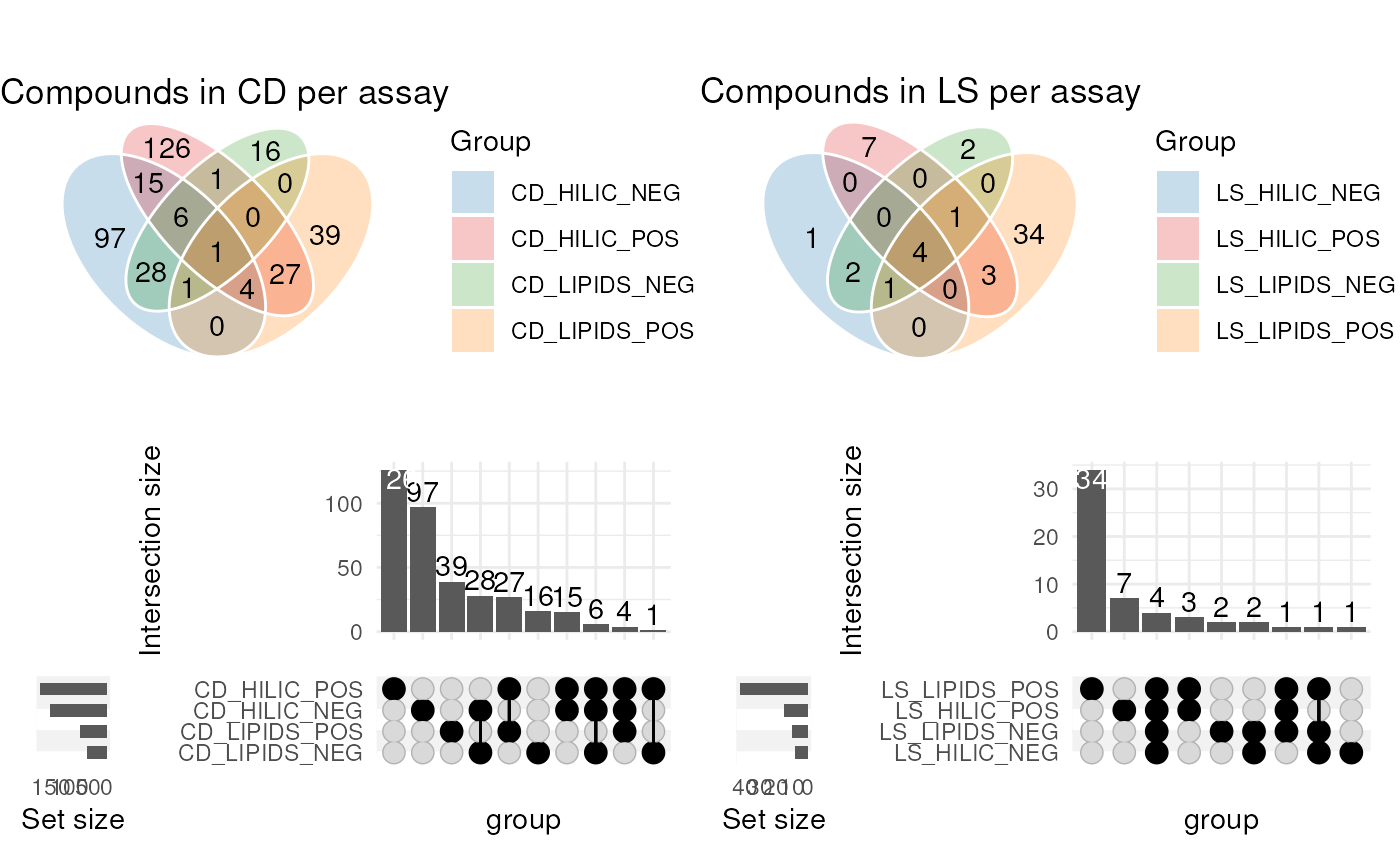
The diagram for CD shows the largest amount of overlap is between assays with the same ion mode.
For LS the number of annotations is quite small, so the diagram is less informative. However, we are clearly detecting a larger number of annotations in the LIPIDS assays, which is to be expected as the LS software is designed to annotate lipids molecules.
Here the annotation_venn_chart and
annotation_upset_chart objects were used to compare the
same column across several annotation_tables. The same
objects can also compare groups from within the same table, which we
will explore later.
First, we need to combine the CD and LS tables.
Combining Annotation Sources
In this workflow step we combine the imported assay tables from each assay and annotation source vertically into a single annotation table.
The combine_tables object can be used for this step.
Combining tables from the same source (e.g. the CD table for each assay)
is straight forward as all tables have the same columns.
When combining different sources the combine_tables
object provides input parameters that allow you to combine and select
columns from different sources into new columns with the same
information. For example the adduct column in CD is called
“Ion” and in LS it is called “LipidIon”; we can combine these columns
into a new column called “adduct”.
Here we specify that all columns should be retained from both tables, padding with NA if not present; columns with the same name are automatically merged.
# get all the cleaned annotation tables in one list
all_source_tables <- lapply(c(CD, LS), predicted)

# prepare to merge
combine_workflow <-
    combine_sources(
        source_list = all_source_tables,
        matching_columns = c(
            name = "LipidName",
            name = "compound",
            adduct = "ion",
            adduct = "LipidIon"
        ),
        keep_cols = ".all",
        source_col = "annotation_table",
        exclude_cols = NULL,
        tag = "combined"
    )

# merge
combine_workflow <- model_apply(combine_workflow, lcms_table())

# show
predicted(combine_workflow)
#> A "annotation_source" object
#> ----------------------------
#> name:          combined
#> description:   A source created by combining two or more sources
#> input params:  tag, data, source
#> annotations:   912 rows x 28 columns
Now that the tables have been combined we can explore the table using charts. For example, we visualise the number of annotations for each assay from both sources.
C <- annotation_pie_chart(
    factor_name = "assay",
    label_rotation = FALSE,
    label_location = "outside",
    label_type = "percent",
    legend = TRUE,
    centre_radius = 0.5,
    centre_label = ".total"
)

chart_plot(C, predicted(combine_workflow)) +
    ggtitle("Annotations per assay") +
    theme(plot.margin = unit(c(1, 1.5, 1, 1.5), "cm")) +
    guides(fill = guide_legend(title = "Assay"))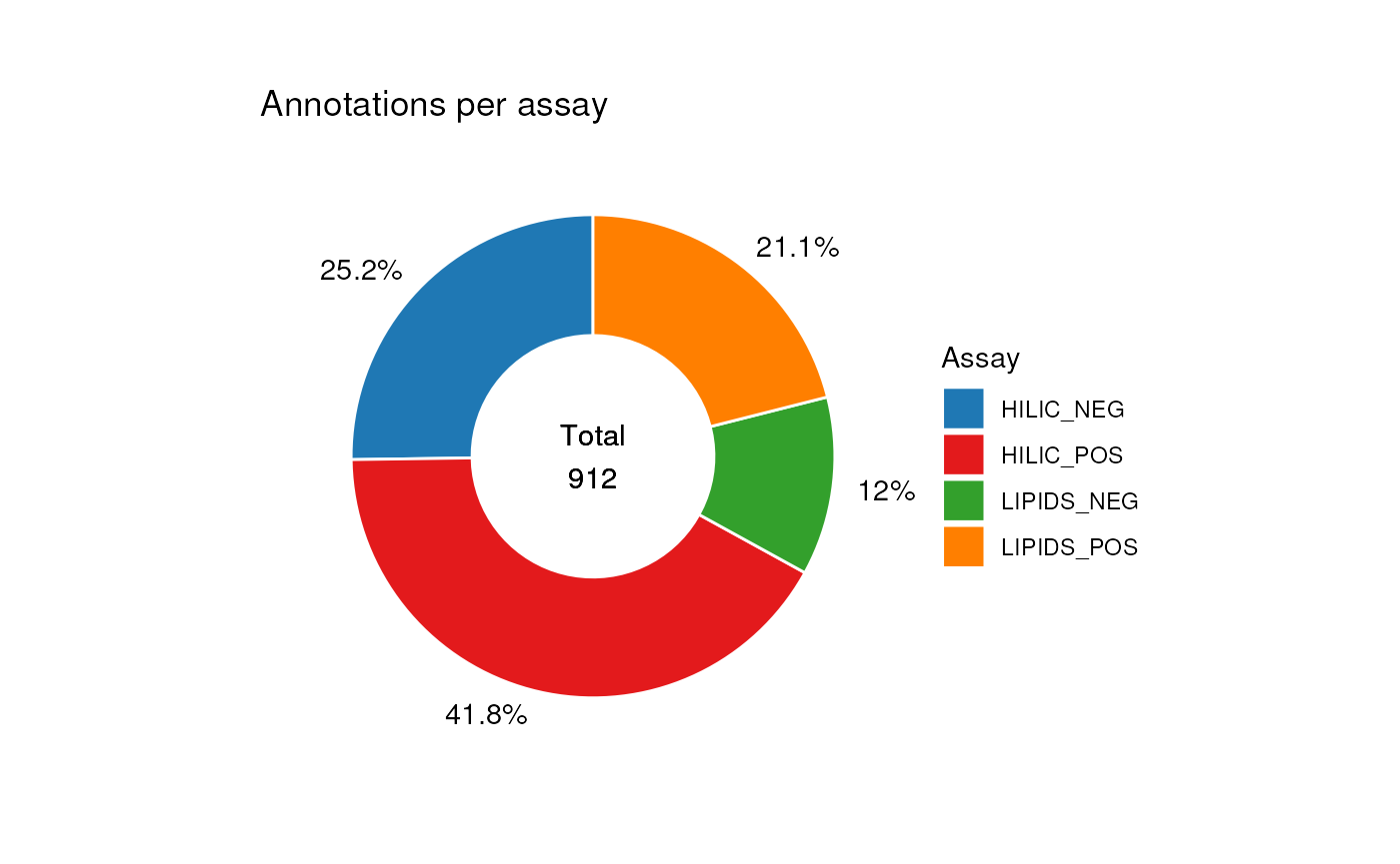
In this next example we compare the number of annotations from each source.
# change to plot source_name column
C$factor_name <- "source_name"
chart_plot(C, predicted(combine_workflow)) +
    ggtitle("Annotations per source") +
    theme(plot.margin = unit(c(1, 1.5, 1, 1.5), "cm")) +
    guides(fill = guide_legend(title = "Source"))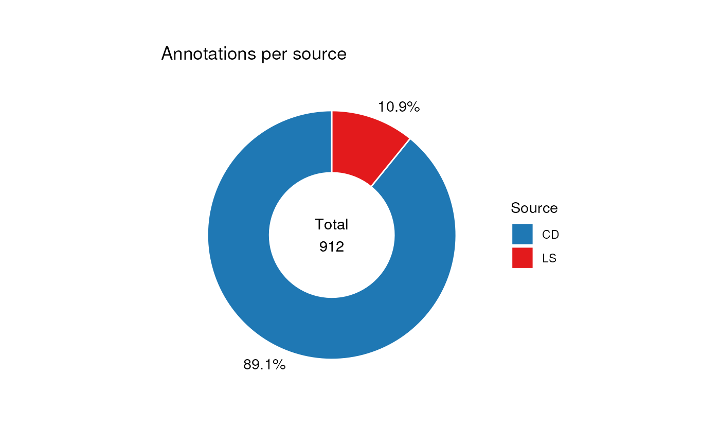
Adding identifiers
Ultimately we would like to compare the annotations detected using our software sources to the list of standard we included in the samples. Comparing the two tables using metabolite names is less than ideal, because different sources might use different synonyms for the same molecular structure.
To overcome this it is much better to compare the tables using
molecular identifiers such as InChIKey, which are unique to the
molecule. MetMashR includes a number of workflow steps that
allow us to look up identifiers from various databases, either stored
locally, or in online databases such as PubChem by using their REST
API.
For this vignette we use cached results so that we don’t overburden the api; in practice you would create your own (see [TODO]).
# import cached results
inchikey_cache <- rds_database(
    source = file.path(
        system.file("cached", package = "MetMashR"),
        "pubchem_inchikey_mtox_cache.rds"
    )
)

id_workflow <-
    pubchem_property_lookup(
        query_column = "name",
        search_by = "name",
        suffix = "",
        property = "InChIKey",
        records = "best",
        cache = inchikey_cache
    )

id_workflow <- model_apply(id_workflow, predicted(combine_workflow))
Improving ID coverage
The ID’s obtained in the previous section were obtained by queries based on the molecule name.
Molecule names can contain a number of special characters, and follow different nomenclatures when constructing the name, as well as abbreviations and naming conventions.
It useful therefore to apply some kind of “molecule name normalisation” to account for these properties of molecule names.
We can use the normalise_strings MetMashR object to do
this. This object has a dictionary parameter that takes the
form of a list of lists.
Each sub-list contains a pattern to be matched and a replacement. In the example workflow below we include a number of definitions in our dictionary:
- Update compounds starting with “NP” to start “Compound NP” as this is how they are recorded in PubChem.
- Replace any molecule name containing a ? with NA, as this indicates ambiguity in the annotation.
- Remove abbreviations from molecule names e.g. “adenosine triphosphate (ATP)” should have the “(ATP)” part removed.
- Replace some shorthand names with more formal names that are more likely to result in a match to a PubChem compound.
- Remove optical properties from racemic compounds e.g. D-(+)-Glucose becomes D-Glucose.
- Replace Greek characters with their Romanised names.
Both the Greek and racemic dictionaries are provided by MetMashR for convenience.
In steps 2 and 3 of the workflow we submit these normalised names to the PubChem API and to OPSIN. By utlilising serveral API’s we can maximise the number of molecules we obtain an InChIKey for.
In the final step we merge the three columns of identifiers, giving priority to OPSIN, which is based on deconstructing the molecule name into its component parts. If there is no result from OPSIN then a PubChem search based on the normalised names is prioritised over a PubChem search using the non-normalised names.
# prepare cached results for vignette
inchikey_cache2 <- rds_database(
    source = file.path(
        system.file("cached", package = "MetMashR"),
        "pubchem_inchikey_mtox_cache2.rds"
    )
)
inchikey_cache3 <- rds_database(
    source = file.path(
        system.file("cached", package = "MetMashR"),
        "pubchem_inchikey_mtox_cache3.rds"
    )
)

N <- normalise_strings(
    search_column = "name",
    output_column = "normalised_name",
    dictionary = c(
        # custom dictionary
        list(
            # replace "NP" with "Compound NP"
            list(pattern = "^NP-", replace = "Compound NP-"),
            # replace ? with NA, since this is ambiguous
            list(pattern = "?", replace = NA, fixed = TRUE),
            # remove terms in trailing brackets e.g." (ATP)"
            list(pattern = "\\ \\([^\\)]*\\)$", replace = ""),
            # replace known abbreviations
            list(
                pattern = "(+/-)9-HpODE",
                replace = "9-hydroperoxy-10E,12Z-octadecadienoic acid",
                fixed = TRUE
            ),
            list(
                pattern = "(+/-)19(20)-DiHDPA",
                replace =
                    "19,20-dihydroxy-4Z,7Z,10Z,13Z,16Z-docosapentaenoic acid",
                fixed = TRUE
            )
        ),
        # replace greek characters
        greek_dictionary,
        # remove racemic properties
        racemic_dictionary
    )
) +
    pubchem_property_lookup(
        query_column = "normalised_name",
        search_by = "name",
        suffix = "_norm",
        property = "InChIKey",
        records = "best",
        cache = inchikey_cache2
    ) +
    opsin_lookup(
        query_column = "normalised_name",
        suffix = "_opsin",
        output = "stdinchikey",
        cache = inchikey_cache3
    ) +
    prioritise_columns(
        column_names = c("stdinchikey_opsin", "InChIKey_norm", "InChIKey"),
        output_name = "inchikey",
        source_name = "inchikey_source",
        clean = TRUE
    )

N <- model_apply(N, predicted(id_workflow))
We can explore the impact of these workflow steps using Venn and Pie charts to compare the results before/after the workflow.
In this Venn diagram we show the overlap between the InChIKey identifiers obtained from the three queries. It can be seen that normalising the names resulted in 37 identifiers that we were unable to obtain without normalisation.
The use of OPSIN then added a further 31 identifiers. The column of combined identifers therefore contains
# venn inchikey columns
C <- annotation_venn_chart(
    factor_name = c("InChIKey", "InChIKey_norm", "stdinchikey_opsin"),
    line_colour = "white",
    fill_colour = ".group",
    legend = TRUE,
    labels = FALSE
)
chart_plot(C, predicted(N[3])) +
    guides(
        fill = guide_legend(title = "Source"),
        colour = guide_legend(title = "Source")
    ) +
    theme(plot.margin = unit(c(1, 1.5, 1, 1.5), "cm"))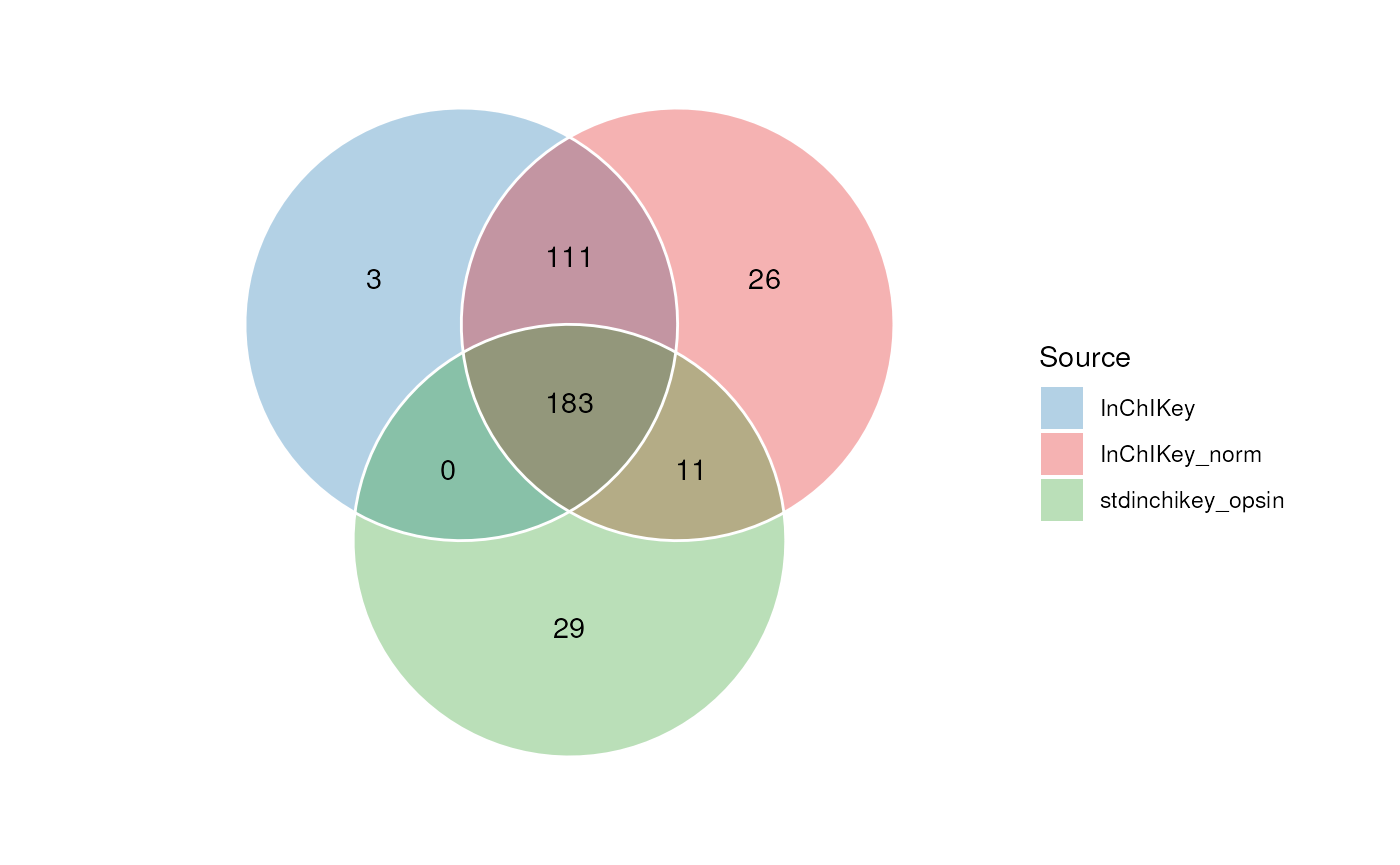
Due to complexity, Venn charts are limited to 7 sets. UpSet plots are an alternative chart than can accomodate many more sets. Each veritcal bar in the UpSet plot corresponds to a region in the venn diagram.
# upset inchikey columns
C <- annotation_upset_chart(
    factor_name = c("InChIKey", "InChIKey_norm", "stdinchikey_opsin"),
    min_size = 0,
    n_intersections = 10
)
chart_plot(C, predicted(N[3]))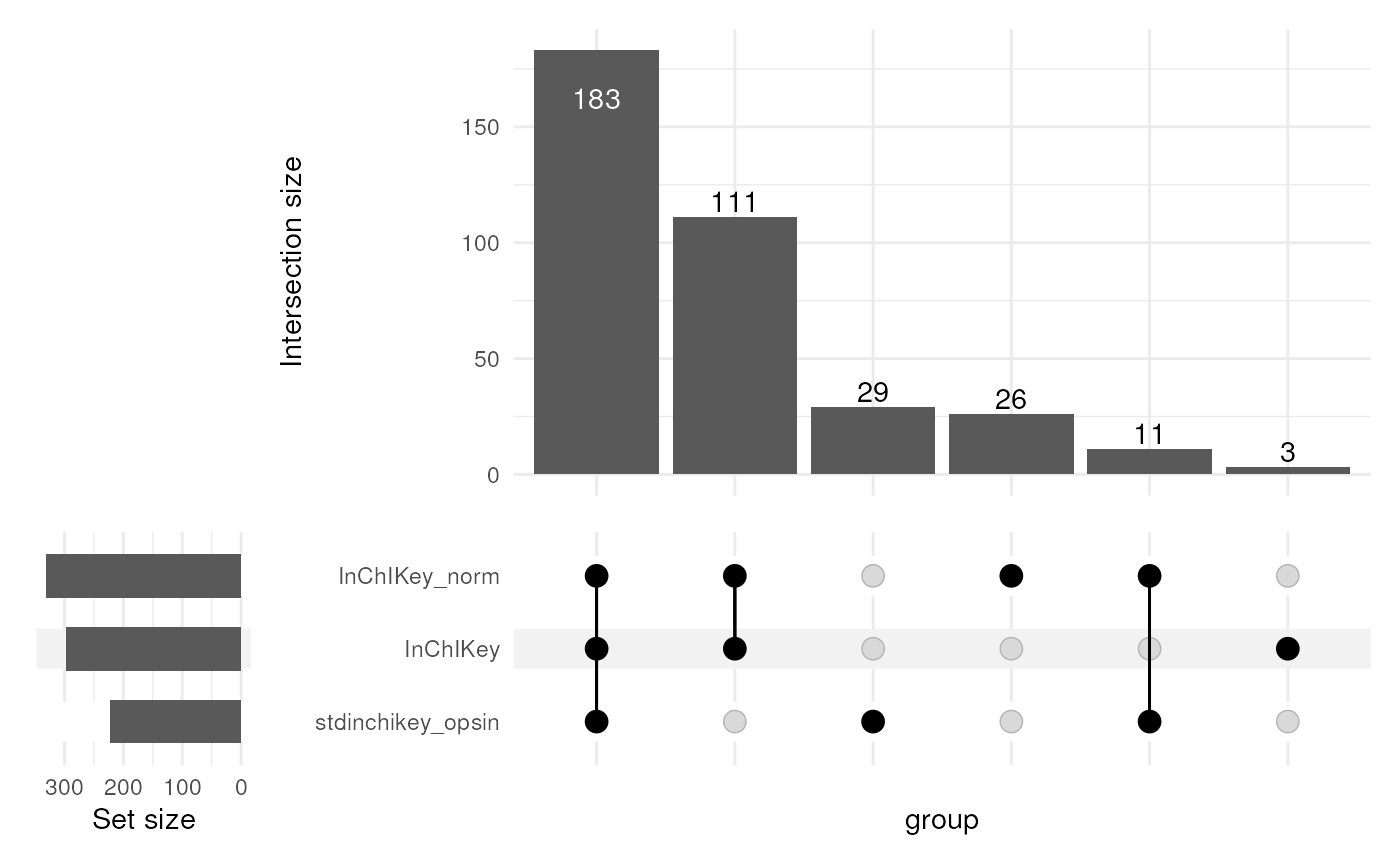
In the next chart we visualise the proportion of annotations from each query, after prioritisation and merging has taken place.
Note that in this case some of the identifiers might be the same if e.g. the same molecule is present in multiple rows. You can see that in the end only a small proportion (12.1%) of the identifiers are from the least reliable query based on the non-normalised name.
# pie source of inchikey
C <- annotation_pie_chart(
    factor_name = "inchikey_source",
    label_rotation = FALSE,
    label_location = "outside",
    label_type = "percent",
    legend = TRUE,
    centre_radius = 0.5,
    centre_label = ".total",
    count_na = TRUE
)
chart_plot(C, predicted(N)) +
    guides(
        fill = guide_legend(title = "Source"),
        colour = guide_legend(title = "Source")
    ) +
    theme(plot.margin = unit(c(1, 1.5, 1, 1.5), "cm"))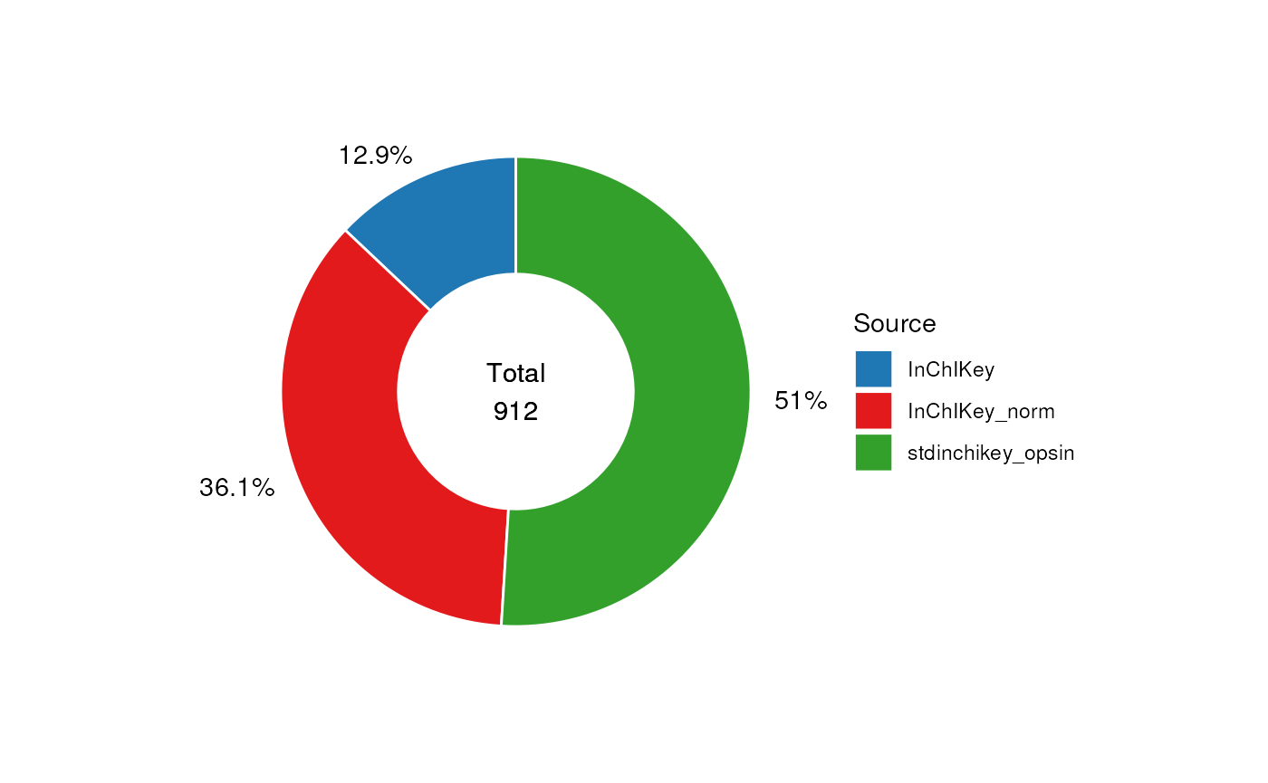
To keep the records with the highest confidence identifiers We can
remove the annotations based on the name query using the
filter_labels object.
# prepare workflow
FL <- filter_labels(
    column_name = "inchikey_source",
    labels = "InChIKey",
    mode = "exclude"
)
# apply
FF <- model_apply(FL, predicted(N))

# print summary
predicted(FF)
#> A "annotation_source" object
#> ----------------------------
#> name:          combined
#> description:   A source created by combining two or more sources
#> input params:  tag, data, source
#> annotations:   465 rows x 33 columns
Comparison with the true mixtures
In this section we compare the annotated features with the table of standards known to be included in each of the mixtures.
Importing the standard mixture tables
The first step is to import the tables of standards for each mixture.
The data has ready been saved as an RDS file so we can use
rds_database to import it.
# prepare object
R <- rds_database(
    source = file.path(
        system.file("extdata", package = "MetMashR"),
        "standard_mixtures.rds"
    ),
    .writable = FALSE
)

# read
R <- read_source(R)
The standards table contains a list of metabolites and the the mixture they were included in. It also contains some manually curated data providing m/z and retention time of the metabolite, which assay it was observed in and the adduct.
Identifiers for the standards
The standards table provides HMDB identifiers for each metabolite, but our preference is to work with InChIkey. So our first task is to obtain InChiKey for the standards.
The standards are based on the MTox700+ database (see [TODO]), so we
can import MTox700+ and use it to obtain InChIKey identifiers by
matching the the HMBD identifiers. An alternative might be to use
hmdb_lookup and/or
pubchem_property_lookup.
# convert standard mixtures to source, then get inchikey from MTox700+
SM <- import_source() +
    filter_na(
        column_name = "rt"
    ) +
    filter_na(
        column_name = "median_ms2_scans"
    ) +
    filter_na(
        column_name = "mzcloud_id"
    ) +
    filter_range(
        column_name = "median_ms2_scans",
        upper_limit = Inf,
        lower_limit = 0,
        equal_to = TRUE
    ) +
    database_lookup(
        query_column = "hmdb_id",
        database_column = "hmdb_id",
        database = MTox700plus_database(),
        include = "inchikey",
        suffix = "",
        not_found = NA
    ) +
    id_counts(
        id_column = "inchikey",
        count_column = "inchikey_count",
        count_na = FALSE
    )
# apply
SM <- model_apply(SM, R)
In this next plot we show the overlap in standards for each assay detected by manual observation.
C <- annotation_venn_chart(
    factor_name = "inchikey",
    group_column = "ion_mode",
    line_colour = "white",
    fill_colour = ".group",
    legend = TRUE,
    labels = FALSE
)

## plot
chart_plot(C, predicted(SM))
Comparison of standards and annotations
Now that we have both the annotations and the standards we can look at overlap between the identifiers in both sources, and begin to assess the ability of the annotation software annotate the standards.
Here we plot a venn diagram showing the overlap in identifiers.
# get processed data
AN <- predicted(FF)
AN$tag <- "Annotations"
sM <- predicted(SM)
sM$tag <- "Standards"

# prepare chart
C <- annotation_venn_chart(
    factor_name = "inchikey",
    line_colour = "white",
    fill_colour = ".group"
)

# plot
chart_plot(C, sM, AN) + ggtitle("All assays, all sources")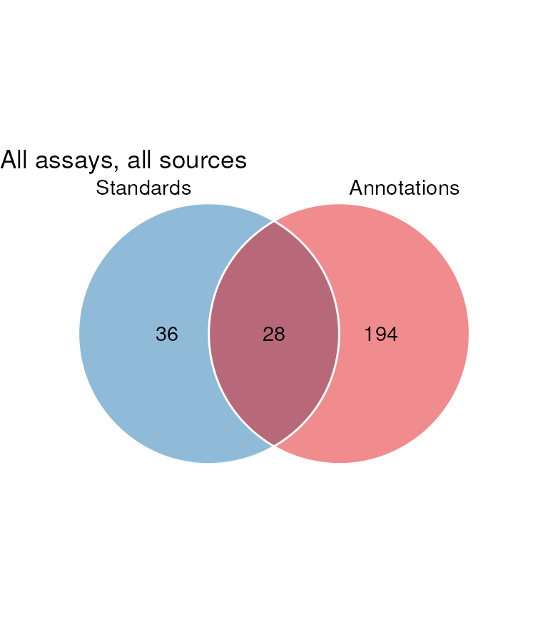
It can been seen that there is a large number of annotations not present in the standard. These are false positives.
In the next plot we show similar Venn diagrams but for each assay individually. These are followed by a 4-set Venn diagram that shows the overlap between annotations from each assay that matched to a standard.
G <- list()
VV <- list()
for (k in c("HILIC_NEG", "HILIC_POS", "LIPIDS_NEG", "LIPIDS_POS")) {
    wf <- filter_labels(
        column_name = "assay",
        labels = k,
        mode = "include"
    )
    wf1 <- model_apply(wf, AN)
    wf$column_name <- "ion_mode"
    wf2 <- model_apply(wf, sM)
    G[[k]] <- chart_plot(C, predicted(wf2), predicted(wf1))

    V <- filter_venn(
        factor_name = "inchikey",
        tables = list(predicted(wf1)),
        levels = "Standards/Annotations",
        mode = "include"
    )
    V <- model_apply(V, predicted(wf2))
    VV[[k]] <- predicted(V)
    VV[[k]]$tag <- k
}
r1 <- cowplot::plot_grid(
    plotlist = G, nrow = 2,
    labels = c("HILIC_NEG", "HILIC_POS", "LIPIDS_NEG", "LIPIDS_POS")
)

cowplot::plot_grid(r1, chart_plot(C, VV), nrow = 2, rel_heights = c(1, 0.5))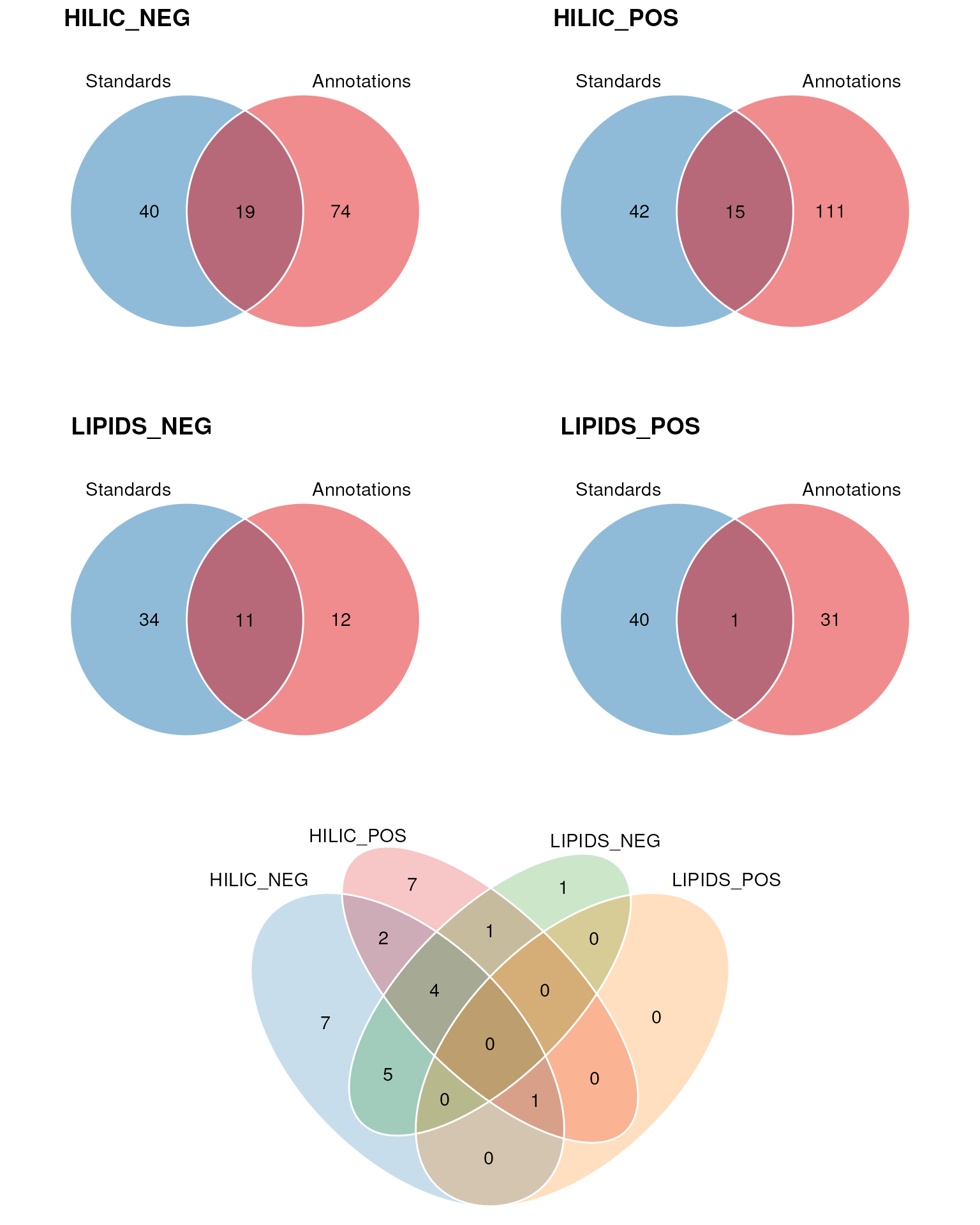
The majority of the standards were correctly annotated in the HILIC_NEG assay.
In the next plot we compare the overlap in InChIKey for each source.
G <- list()
for (k in c("CD", "LS")) {
    wf <- filter_labels(
        column_name = "source_name",
        labels = k,
        mode = "include"
    )
    wf1 <- model_apply(wf, AN)

    G[[k]] <- chart_plot(C, sM, predicted(wf1))
}
cowplot::plot_grid(plotlist = G, nrow = 1, labels = c("CD", "LS"))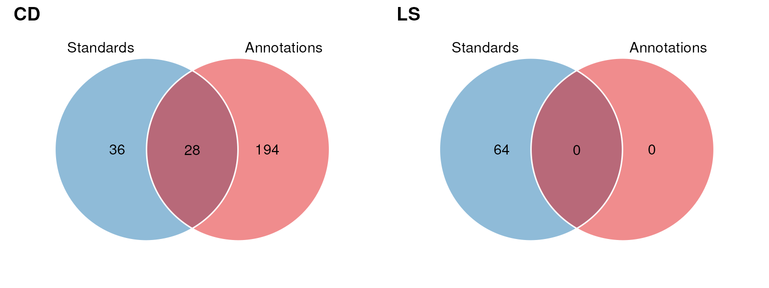
Session Info
sessionInfo()
#> R version 4.4.1 (2024-06-14)
#> Platform: x86_64-pc-linux-gnu
#> Running under: Ubuntu 22.04.5 LTS
#>
#> Matrix products: default
#> BLAS:   /usr/lib/x86_64-linux-gnu/openblas-pthread/libblas.so.3
#> LAPACK: /usr/lib/x86_64-linux-gnu/openblas-pthread/libopenblasp-r0.3.20.so;  LAPACK version 3.10.0
#>
#> locale:
#>  [1] LC_CTYPE=en_US.UTF-8       LC_NUMERIC=C
#>  [3] LC_TIME=en_US.UTF-8        LC_COLLATE=en_US.UTF-8
#>  [5] LC_MONETARY=en_US.UTF-8    LC_MESSAGES=en_US.UTF-8
#>  [7] LC_PAPER=en_US.UTF-8       LC_NAME=C
#>  [9] LC_ADDRESS=C               LC_TELEPHONE=C
#> [11] LC_MEASUREMENT=en_US.UTF-8 LC_IDENTIFICATION=C
#>
#> time zone: UTC
#> tzcode source: system (glibc)
#>
#> attached base packages:
#> [1] stats     graphics  grDevices utils     datasets  methods   base
#>
#> other attached packages:
#> [1] DT_0.33              dplyr_1.1.4          structToolbox_1.18.0
#> [4] ggplot2_3.5.1        MetMashR_1.0.0       struct_1.18.0
#> [7] BiocStyle_2.34.0
#>
#> loaded via a namespace (and not attached):
#>  [1] tidyselect_1.2.1            blob_1.2.4
#>  [3] farver_2.1.2                filelock_1.0.3
#>  [5] fastmap_1.2.0               BiocFileCache_2.14.0
#>  [7] digest_0.6.37               lifecycle_1.0.4
#>  [9] RSQLite_2.3.7               magrittr_2.0.3
#> [11] compiler_4.4.1              rlang_1.1.4
#> [13] sass_0.4.9                  tools_4.4.1
#> [15] utf8_1.2.4                  yaml_2.3.10
#> [17] knitr_1.48                  S4Arrays_1.6.0
#> [19] labeling_0.4.3              htmlwidgets_1.6.4
#> [21] bit_4.5.0                   curl_5.2.3
#> [23] ontologyIndex_2.12          sp_2.1-4
#> [25] DelayedArray_0.32.0         plyr_1.8.9
#> [27] abind_1.4-8                 withr_3.0.2
#> [29] purrr_1.0.2                 BiocGenerics_0.52.0
#> [31] desc_1.4.3                  grid_4.4.1
#> [33] stats4_4.4.1                fansi_1.0.6
#> [35] colorspace_2.1-1            scales_1.3.0
#> [37] SummarizedExperiment_1.36.0 cli_3.6.3
#> [39] rmarkdown_2.28              crayon_1.5.3
#> [41] ragg_1.3.3                  generics_0.1.3
#> [43] httr_1.4.7                  DBI_1.2.3
#> [45] cachem_1.1.0                stringr_1.5.1
#> [47] zlibbioc_1.52.0             ggthemes_5.1.0
#> [49] BiocManager_1.30.25         XVector_0.46.0
#> [51] matrixStats_1.4.1           vctrs_0.6.5
#> [53] Matrix_1.7-1                jsonlite_1.8.9
#> [55] bookdown_0.41               patchwork_1.3.0
#> [57] IRanges_2.40.0              S4Vectors_0.44.0
#> [59] bit64_4.5.2                 systemfonts_1.1.0
#> [61] crosstalk_1.2.1             jquerylib_0.1.4
#> [63] tidyr_1.3.1                 ggVennDiagram_1.5.2
#> [65] glue_1.8.0                  pkgdown_2.1.1.9000
#> [67] cowplot_1.1.3               stringi_1.8.4
#> [69] gtable_0.3.6                RVenn_1.1.0
#> [71] GenomeInfoDb_1.42.0         GenomicRanges_1.58.0
#> [73] UCSC.utils_1.2.0            ComplexUpset_1.3.3
#> [75] munsell_0.5.1               tibble_3.2.1
#> [77] pillar_1.9.0                htmltools_0.5.8.1
#> [79] GenomeInfoDbData_1.2.13     dbplyr_2.5.0
#> [81] R6_2.5.1                    textshaping_0.4.0
#> [83] evaluate_1.0.1              lattice_0.22-6
#> [85] Biobase_2.66.0              highr_0.11
#> [87] openxlsx_4.2.7.1            memoise_2.0.1
#> [89] bslib_0.8.0                 Rcpp_1.0.13
#> [91] zip_2.3.1                   gridExtra_2.3
#> [93] SparseArray_1.6.0           xfun_0.48
#> [95] fs_1.6.4                    MatrixGenerics_1.18.0
#> [97] pkgconfig_2.0.3