Exploring the MTox700+ library
Gavin Rhys Lloyd
2024-11-05
Source:vignettes/exploring_mtox.Rmd
exploring_mtox.Rmd# Getting Started The latest versions of struct and
MetMashR that are compatible with your current R version
can be installed using BiocManager.
# install BiocManager if not present
if (!requireNamespace("BiocManager", quietly = TRUE)) {
    install.packages("BiocManager")
}

# install MetMashR and dependencies
BiocManager::install("MetMashR")
Once installed you can activate the packages in the usual way:
# load the packages
library(MetMashR)
library(ggplot2)
library(structToolbox)
library(dplyr)
library(DT)
Introduction
MTox700+ is a list of toxicologically relevant metabolites derived from publications, public databases and relevant toxicological assays.
In this vignette we import the MTox700+ database and combine.merge and “mash” it with other databases to explore its contents and it’s coverage of chemical, biological and toxicological space.
Importing the MTox700+ database
The MTox700+ database can be imported using the
MTox700plus_database object. It can be imported to a
data.frame using the read_database method.
# prep object
MT <- MTox700plus_database(
    version = "latest",
    tag = "MTox700+"
)

# import
df <- read_database(MT)

# show contents
.DT(df)
# prepare workflow that uses MTox700+ as a source
M <-
    import_source() +
    trim_whitespace(
        column_name = ".all",
        which = "both",
        whitespace = "[\\h\\v]"
    )

# apply
M <- model_apply(M, MT)
Exploring the chemical space
The chemical (or “metabolite”) space covered by the MTox700+ database can be explored in several ways using the data included in the database.
For example, we can generate images of the molecules using the SMILES included in the database. Here we generate images of the first 6 metabolites in the database.
# prepare chart
C <- openbabel_structure(
    smiles_column = "smiles",
    row_index = 1,
    scale_to_fit = FALSE,
    image_size = 300,
    title_column = "metabolite_name",
    view_port = 400
)

# first six
G <- list()
for (k in 1:6) {
    # set row idx
    C$row_index <- k
    # plot
    G[[k]] <- chart_plot(C, predicted(M))
}

# layout
cowplot::plot_grid(plotlist = G, nrow = 2)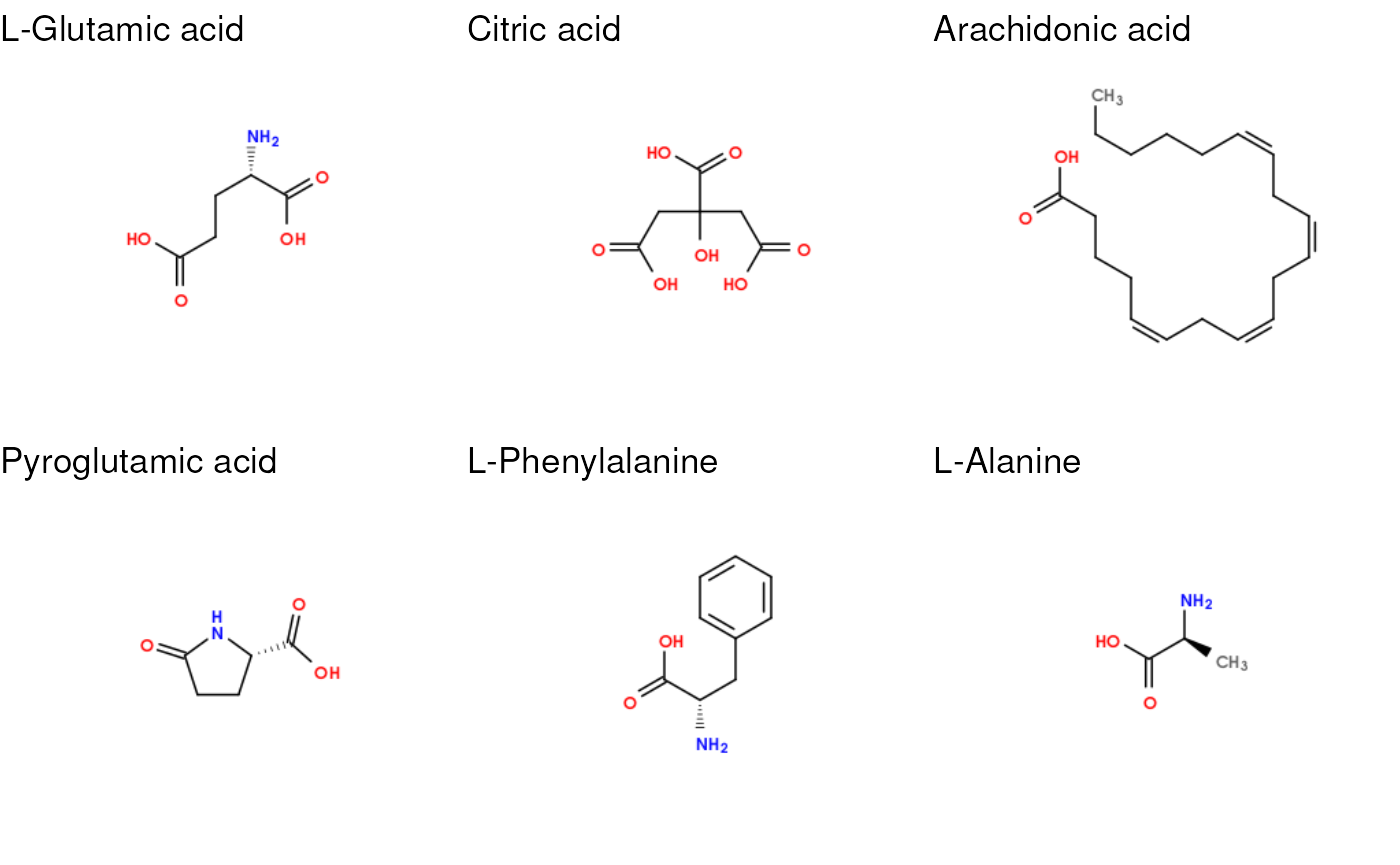
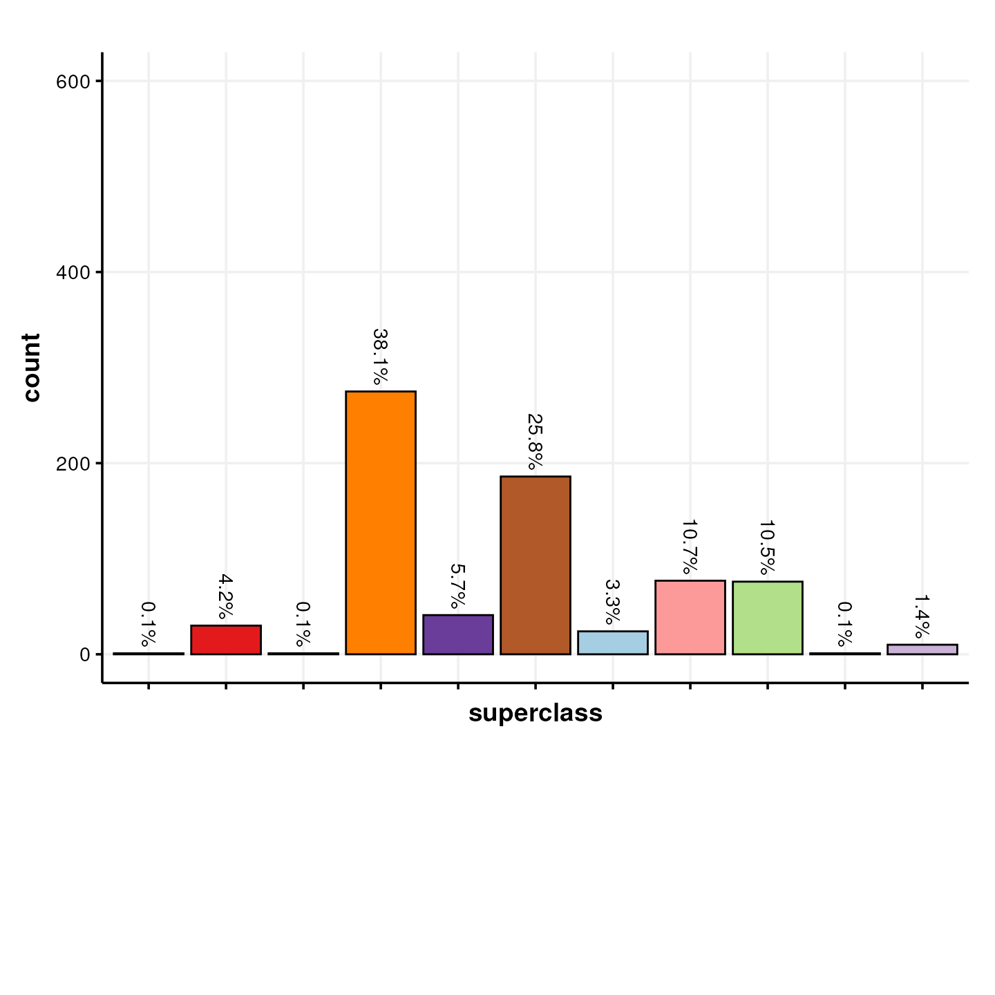
The MTox700+ database also contains information about the structural classification of the metabolites based on ChemOnt (a chemical taxonomy) and ClassyFire (software to compute the taxonomy of a structure) [10.1186/s13321-016-0174-y].
In this plot we show the number of metabolites in the MTox700+ database that are assigned to a “superclass” of molecules.
# initialise chart object
C <- annotation_bar_chart(
    factor_name = "superclass",
    label_rotation = TRUE,
    label_location = "outside",
    label_type = "percent",
    legend = TRUE
)

# plot
g <- chart_plot(C, predicted(M)) + ylim(c(0, 600)) +
    guides(fill = guide_legend(nrow = 6, title = element_blank())) +
    theme(legend.position = "bottom", legend.margin = margin())

# layout
leg <- cowplot::get_legend(g)
cowplot::plot_grid(g + theme(legend.position = "none"), leg,
    nrow = 2,
    rel_heights = c(75, 25)
)
Exploring the biological space
To explore the biological space covered by the metabolites in MTox700+ we need mash the database with additional information about the biological pathways that the metabolites are part of.
We use the PathBank for this
purpose. A struct_database object for PathBank is already
included in MetMashR.
Importing PathBank
MetMashR provides the
PathBank_metabolite_databse object to import the PathBank
database. You can choose to import:
- The “primary” database. This is a smaller version of the database restricted to primary pathways.
- The “complete” database, which includes all pathways in the database.
The “complete” database is a >50mb download, and unzipped is >1Gb. Unzipping and caching of the database is handled by [BiocFileCache].
For the vignette we restrict to the “primary” PathBank database to keep file sizes and downloads to a minimum.
We can use the database in two ways:
- convert it to a source and “mash” it with other sources
- use it as a lookup table to add information to an existing source.
To explore the biological space covered by MetMashR we will do both.
Comparing PathBank and MTox700+
It is useful to visualise the overlap between PathBank and MTox700+. MTox700+ is a much smaller database due to it being a curated list of metabolites with toxicologial relevance, and PathBank is more general.
In th example below we import PathBank as a source, and use a venn diagram to compare the overlap between inchikey identifiers in PathBank and MTox700+.
# object M already contains the MTox700+ database as a source

# prepare PathBank as a source
P <- PathBank_metabolite_database(
    version = "primary",
    tag = "PathBank"
)

# import
P <- read_source(P)

# prepare chart
C <- annotation_venn_chart(
    factor_name = c("inchikey", "InChI.Key"), legend = FALSE,
    fill_colour = ".group",
    line_colour = "white"
)

# plot
g1 <- chart_plot(C, predicted(M), P)

C <- annotation_upset_chart(
    factor_name = c("inchikey", "InChI.Key")
)
g2 <- chart_plot(C, predicted(M), P)
cowplot::plot_grid(g1, g2, nrow = 1, labels = c("Venn diagram", "UpSet plot"))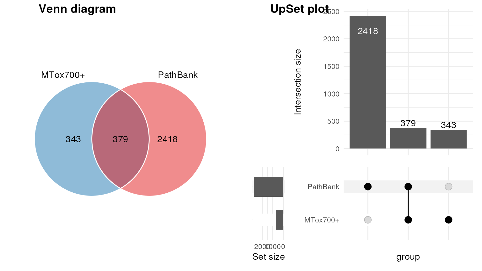
The charts show that less than half of the metabolites in MTox700+ are also present in the PathBank database for primary pathways.
Combining MTox700+ with PathBank
To combine the pathway information in PathBank with the MTox700+
database we can use PathBank as a lookup table based on inchikeys. To do
this we use the database_lookup object.
Note that PathBank is not downloaded a second time; it is automatically retrieved from the cache.
We request a number of columns from PathBank, including pathway information and additional identifiers such as HMBD ID and KEGG ID.
# prepare object
X <- database_lookup(
    query_column = "inchikey",
    database = P$data,
    database_column = "InChI.Key",
    include = c(
        "PathBank.ID", "Pathway.Name", "Pathway.Subject", "Species",
        "HMDB.ID", "KEGG.ID", "ChEBI.ID", "DrugBank.ID", "SMILES"
    ),
    suffix = ""
)

# apply
X <- model_apply(X, predicted(M))
We can now visualise e.g. the subject of the pathways captured by the MTox700+ database.
C <- annotation_bar_chart(
    factor_name = "Pathway.Subject",
    label_rotation = TRUE,
    label_location = "outside",
    label_type = "percent",
    legend = TRUE
)

chart_plot(C, predicted(X)) + ylim(c(0, 17500))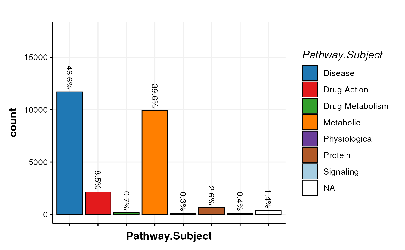
We can see that MTox700+ largely focuses on metabolites related to Disease metabolism and general metabolism, which is concomitant with the database being curated to contain metabolites relevant to toxicology in humans.
Combining records
Metabolites can appear in multiple pathways. The PathBank database therefore contains multiple records for the same metabolite, and the relationship between MTox700+ and PathBank is one-to-many.
After obtaining pathway information from PathBank the new table has many more rows than the original MTox700+ database, as each MTox700+ record has been replicated for each match in the PathBank database.
e.g. after importing MTox700+ the number of records was:
After combing with PathBank the number of records is:
Sometimes it is useful to collapse this information into a single
record per metabolite. We can use the combine_records
object and its helper functions to do this in a MetMashR
workflow.
# prepare object
X <- database_lookup(
    query_column = "inchikey",
    database = P$data,
    database_column = "InChI.Key",
    include = c(
        "PathBank.ID", "Pathway.Name", "Pathway.Subject", "Species",
        "HMDB.ID", "KEGG.ID", "ChEBI.ID", "DrugBank.ID", "SMILES"
    ),
    suffix = ""
) +
    combine_records(
        group_by = "inchikey",
        default_fcn = fuse_unique(" || ")
    )

# apply
X <- model_apply(X, predicted(M))
We have used the .unique helper function so that records
for each inchikey are combined into a single record by only retaining
unique values in each field (column). If there are multiple unique
values for a field then they are combined into a single string using the
” || ” separator.
We can now extract the pathways associated with a particular metabolite. For example Glycolic acid:
The pathways associated with Glycolic acid are:
# print list of pathways
predicted(X)$data$Pathway.Name[w]
#> [1] "Inner Membrane Transport || Glycolate and Glyoxylate Degradation || D-Arabinose Degradation I || Ethylene Glycol Degradation"
Session Info
sessionInfo()
#> R version 4.4.1 (2024-06-14)
#> Platform: x86_64-pc-linux-gnu
#> Running under: Ubuntu 22.04.5 LTS
#>
#> Matrix products: default
#> BLAS:   /usr/lib/x86_64-linux-gnu/openblas-pthread/libblas.so.3
#> LAPACK: /usr/lib/x86_64-linux-gnu/openblas-pthread/libopenblasp-r0.3.20.so;  LAPACK version 3.10.0
#>
#> locale:
#>  [1] LC_CTYPE=en_US.UTF-8       LC_NUMERIC=C
#>  [3] LC_TIME=en_US.UTF-8        LC_COLLATE=en_US.UTF-8
#>  [5] LC_MONETARY=en_US.UTF-8    LC_MESSAGES=en_US.UTF-8
#>  [7] LC_PAPER=en_US.UTF-8       LC_NAME=C
#>  [9] LC_ADDRESS=C               LC_TELEPHONE=C
#> [11] LC_MEASUREMENT=en_US.UTF-8 LC_IDENTIFICATION=C
#>
#> time zone: UTC
#> tzcode source: system (glibc)
#>
#> attached base packages:
#> [1] stats     graphics  grDevices utils     datasets  methods   base
#>
#> other attached packages:
#> [1] DT_0.33              dplyr_1.1.4          structToolbox_1.18.0
#> [4] ggplot2_3.5.1        MetMashR_1.0.0       struct_1.18.0
#> [7] BiocStyle_2.34.0
#>
#> loaded via a namespace (and not attached):
#>  [1] tidyselect_1.2.1            farver_2.1.2
#>  [3] blob_1.2.4                  filelock_1.0.3
#>  [5] fastmap_1.2.0               BiocFileCache_2.14.0
#>  [7] digest_0.6.37               lifecycle_1.0.4
#>  [9] rsvg_2.6.1                  RSQLite_2.3.7
#> [11] magrittr_2.0.3              compiler_4.4.1
#> [13] rlang_1.1.4                 sass_0.4.9
#> [15] tools_4.4.1                 utf8_1.2.4
#> [17] yaml_2.3.10                 knitr_1.48
#> [19] labeling_0.4.3              S4Arrays_1.6.0
#> [21] htmlwidgets_1.6.4           ontologyIndex_2.12
#> [23] bit_4.5.0                   sp_2.1-4
#> [25] curl_5.2.3                  DelayedArray_0.32.0
#> [27] abind_1.4-8                 withr_3.0.2
#> [29] purrr_1.0.2                 BiocGenerics_0.52.0
#> [31] desc_1.4.3                  grid_4.4.1
#> [33] stats4_4.4.1                fansi_1.0.6
#> [35] colorspace_2.1-1            scales_1.3.0
#> [37] SummarizedExperiment_1.36.0 cli_3.6.3
#> [39] rmarkdown_2.28              crayon_1.5.3
#> [41] ragg_1.3.3                  generics_0.1.3
#> [43] httr_1.4.7                  DBI_1.2.3
#> [45] cachem_1.1.0                stringr_1.5.1
#> [47] zlibbioc_1.52.0             ggthemes_5.1.0
#> [49] BiocManager_1.30.25         XVector_0.46.0
#> [51] matrixStats_1.4.1           vctrs_0.6.5
#> [53] Matrix_1.7-1                jsonlite_1.8.9
#> [55] bookdown_0.41               patchwork_1.3.0
#> [57] IRanges_2.40.0              S4Vectors_0.44.0
#> [59] bit64_4.5.2                 magick_2.8.5
#> [61] crosstalk_1.2.1             systemfonts_1.1.0
#> [63] tidyr_1.3.1                 jquerylib_0.1.4
#> [65] ggVennDiagram_1.5.2         glue_1.8.0
#> [67] ChemmineOB_1.44.0           pkgdown_2.1.1.9000
#> [69] cowplot_1.1.3               stringi_1.8.4
#> [71] gtable_0.3.6                RVenn_1.1.0
#> [73] GenomeInfoDb_1.42.0         GenomicRanges_1.58.0
#> [75] UCSC.utils_1.2.0            ComplexUpset_1.3.3
#> [77] munsell_0.5.1               tibble_3.2.1
#> [79] pillar_1.9.0                htmltools_0.5.8.1
#> [81] GenomeInfoDbData_1.2.13     dbplyr_2.5.0
#> [83] R6_2.5.1                    textshaping_0.4.0
#> [85] evaluate_1.0.1              lattice_0.22-6
#> [87] Biobase_2.66.0              highr_0.11
#> [89] memoise_2.0.1               bslib_0.8.0
#> [91] Rcpp_1.0.13                 gridExtra_2.3
#> [93] SparseArray_1.6.0           xfun_0.48
#> [95] fs_1.6.4                    MatrixGenerics_1.18.0
#> [97] pkgconfig_2.0.3