Introduction
MetMashR is an R package designed to facilitate the cleaning, filtering and combining of annotations from different sources. MetMashR defines an”annotation source” as a piece of software, proprietary or otherwise, that takes the raw input of an analytical instrument and attempts to assign molecule names to the peaks in the data, usually by comparison to a library. MetMashR was primarily designed for use with metabolomics data measured by LCMS (hence “metabolite” in the package name) but could be extended to include other platforms (e.g. NMR, DIMS etc.), or other analytical approaches.
In this vignette we describe commonly used annotation workflow steps and show how to use them in detail.
Statistics in R using Class Templates (struct)
All of the objects defined in MetMashR use or extend the class templates defined by the struct package. Although originally intended for statistics applications, the templates in the struct package have proven to be adaptable to many different scenarios and types of analysis/workflow step.
The use of struct templates allows workflow steps to be applied in sequence and intermediate outputs to be retained for further analysis if required. The templates include ontology definitions for both the object and its input/output parameters. This makes the workflows more “FAIR” which is critical alongside FAIR data to making workflows repeatable, transparent and reproducible.
A general summary of extending struct templates is provided in the package vignette.
Getting Started
The latest versions of struct and MetMashR that are compatible with your current R version can be installed using BiocManager.
# install BiocManager if not present
if (!requireNamespace("BiocManager", quietly = TRUE)) {
    install.packages("BiocManager")
}

# install MetMashR and dependencies
BiocManager::install("MetMashR")
Once installed you can activate the packages in the usual way:
# load the packages
library(struct)
library(MetMashR)
library(metabolomicsWorkbenchR)
library(ggplot2)
Annotation Sources
annotation_source objects are the dataset used by all
MetMashR
workflow steps. If you have used our structToolbox
package before, then annotation sources used equivalently to
DatasetExperiment objects, except that they hold a single
data.frame of metabolite annotation data.
The annotation_source object is not very specific, and
not intended for general use. Instead we have extended them to two main
types of source:
annotation_tableannotation_database
Although all annotation_sources contain a single a
data.frame, the intended use of annotation_table and
annotation_database is different.
Annotation Tables
A annotation_table is defined by us as a
data.frame of metabolite annotations for experimentally
collected data. For example, we have provided lcms_table
objects which ensure that both m/z and retention time data is included
in the data.frame for LCMS data. Usually this table of annotations is
acquired after the application software to generate annotations for an
experimental data set.
Note:
It is not the aim of MetMashR
to generate these annotations. Instead we aim to provide tools to
process, filter, clean and otherwise “mash” this table of annotations
generated elsewhere.
annotation_table objects should have a
read_source method specific to the source. For example the
read_source method for ls_source object reads
in the exported data file from LipidSearch by stripping the header and
parsing the rest of the file into a table.
# prepare source object
AT <- ls_source(
    source = system.file(
        paste0("extdata/MTox/LS/MTox_2023_HILIC_POS.txt"),
        package = "MetMashR"
    )
)

# read source
AT <- read_source(AT)

# show info
AT
#> A "ls_source" object
#> --------------------
#> name:          LCMS table
#> description:   An LCMS table extends [`annotation_table()`] to represent annotation data for an LCMS
#>                  experiment. Columns representing m/z and retention time are required for an
#>                  `lcms_table`.
#> input params:  mz_column, rt_column
#> annotations:   62 rows x 12 columns
The imported annotation_table object is compatible with
MetMashR workflow steps.
Annotation Databases
An annotation_database is a table of additional
metabolite meta data. For example it might contain identifiers and/or
InChIKeys for different metabolites. Usually (but not always) this table
is used in a read-only fashion and is used to augment an
annotation_table with additional information.
Like other sources, annotation_database objects have a
read_source method specific to the database.
# prepare source object
MT <- MTox700plus_database()

# read
MT <- read_source(MT)

# show
MT
#> A "MTox700plus_database" object
#> -------------------------------
#> name:          MTox700plus_database
#> description:   Imports the MTox700+ database, which is made available under the ODC Attribution License.
#>                  MTox700+ is a list of toxicologically relevant metabolites derived from
#>                  publications, public databases and relevant toxicological assays.
#> input params:  version
#> annotations:   722 rows x 15 columns
annotation_database objects also have a
read_database method to read the table directly to a
data.frame.
# prepare source object
MT <- MTox700plus_database()

# read to data.frame
df <- read_database(MT)

# show
.DT(df)
Some annotation_database objects also have a
write_database method, that allows you to update the table
on disk. For example, in MetMashR
the rds_database has a write_database method.
It is useful in combination with rest_api objects to cache
results and reduce the number of requests to the api.
Cached databases
An annotation_database class has been included that uses
functionality provided by BiocFileCache. Although not used
directly, many of the annotation_database objects provided
by MetMashR extend the BiocFileCache_database
object so that the web resources they retrieve are cached locally.
Annotation Mashing
We define annotation mashing as the importing, cleaning, filtering and combining of multiple annotation sources. This is useful for metabolomics datasets where there might be several assays and/or sources of information/annotations.
Importing sources
Although annotation_sources all have a
read_source method, it is convenient to be able to read in
a source as part of a workflow.
The import_source model (workflow step) allows you to do
this. Note that using this object will replace the existing
annotation_source and is really intended to be used as the
first step in a workflow.
# prepare source object
AT <- ls_source(
    source = system.file(
        paste0("extdata/MTox/LS/MTox_2023_HILIC_POS.txt"),
        package = "MetMashR"
    )
)

# prepare workflow
WF <- import_source()

# apply workflow to annotation source
WF <- model_apply(WF, AT)

# show
predicted(WF)
#> A "ls_source" object
#> --------------------
#> name:          LCMS table
#> description:   An LCMS table extends [`annotation_table()`] to represent annotation data for an LCMS
#>                  experiment. Columns representing m/z and retention time are required for an
#>                  `lcms_table`.
#> input params:  mz_column, rt_column
#> annotations:   62 rows x 12 columns
Filtering / Cleaning
MetMashR provides a number of commonly used workflow
steps to filter, clean and process annotation sources. Some of these
steps, such as filter_range are applicable to any
annotation source, while others are specific to a source. For example
mz_rt_match is only applicable to an
lcms_table as it requires that both an m/z and a retention
time column are present. This property is only enforced for
lcms_table objects.
Workflow steps use the model class from
struct. We can build up a workflow by “adding” steps
together to form a model sequence (model_seq). See the
vignettes for struct for more details.
Both models and model sequences can be applied to an
annotation_source objects using the
model_apply method. In this example we import the source,
and then apply a filtering step to remove records with a lower
Grading.
# prepare source object
AT <- ls_source(
    source = system.file(
        paste0("extdata/MTox/LS/MTox_2023_HILIC_POS.txt"),
        package = "MetMashR"
    )
)

# prepare workflow
WF <-
    # step 1 import source from file
    import_source() +
    # step 2 filter the "Grade" column to only include "A" and "B"
    filter_labels(
        column_name = "Grade",
        labels = c("A", "B"),
        mode = "include"
    )

# apply workflow to annotation source
WF <- model_apply(WF, AT)

# show
predicted(WF)
#> A "ls_source" object
#> --------------------
#> name:          LCMS table
#> description:   An LCMS table extends [`annotation_table()`] to represent annotation data for an LCMS
#>                  experiment. Columns representing m/z and retention time are required for an
#>                  `lcms_table`.
#> input params:  mz_column, rt_column
#> annotations:   29 rows x 12 columns
The predicted method returns the processed
annotation_source after applying all steps of the
workflow.
Indexing can also be used with a model sequence to extract the processed annotation source after that step in the workflow.
# source after import and before filtering
predicted(WF[1])
#> A "ls_source" object
#> --------------------
#> name:          LCMS table
#> description:   An LCMS table extends [`annotation_table()`] to represent annotation data for an LCMS
#>                  experiment. Columns representing m/z and retention time are required for an
#>                  `lcms_table`.
#> input params:  mz_column, rt_column
#> annotations:   62 rows x 12 columns
LCMS peak matching
The following methods are restricted to lcms_table
sources:
mz_matchrt_matchmz_rt_matchcalc_ppm_diffcalc_rt_diff
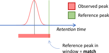
The _match objects align features and annotations by
comparing m/z and/or retention time values between two sources. If the
values fall within a window then this is considered to be a match.
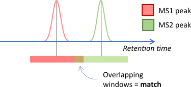
In other cases both sources might be obtained experimentally.
For example when matching MS2 peaks to MS1 peaks. In this case a window
can be applied to both sources, reflecting the uncertainty in
the values for both sources.
REST APIs
MetMashR provides a rest_api object that
implements some base methods to query an api and return a data.frame of
results.
The template has been extended to include api lookup objects for the following:
- ClassyFire
- HMDB
- KEGG
- LipidMaps
- Metabolmics Workbench
- OPSIN
- PubChem
Note these are not necessarily a complete wrapper for all functionality provided by the api; we have only implemented simple wrappers for the most useful parts e.g. querying for molecular identifiers.
The rest_api template object includes the ability to
cache results locally, in order to reduce the number of api queries.
This means a rest_api object can be included in a workflow
and updated as more results are collected over time.
# prepare source object
AT <- ls_source(
    source = system.file(
        paste0("extdata/MTox/LS/MTox_2023_HILIC_POS.txt"),
        package = "MetMashR"
    )
)

# prepare cache
TF <- rds_database(
    source = tempfile()
)

# prepare workflow
WF <-
    # step 1 import source from file
    import_source() +
    # step 2 filter the "Grade" column to only include "A" and "B"
    filter_labels(
        column_name = "Grade",
        labels = c("A", "B"),
        mode = "include"
    ) +
    # step 3 query lipidmaps api for inchikey
    lipidmaps_lookup(
        query_column = "LipidName",
        context = "compound",
        context_item = "abbrev",
        output_item = "inchi_key",
        cache = TF,
        suffix = ""
    )

# apply workflow to annotation source
WF <- model_apply(WF, AT)

# show
predicted(WF)
#> A "ls_source" object
#> --------------------
#> name:          LCMS table
#> description:   An LCMS table extends [`annotation_table()`] to represent annotation data for an LCMS
#>                  experiment. Columns representing m/z and retention time are required for an
#>                  `lcms_table`.
#> input params:  mz_column, rt_column
#> annotations:   39 rows x 14 columns
Note that the cache is stored as an annotation_database
object, and can be used in workflows like any other
annotation_source.
# retrieve cache
TF <- read_source(TF)

# filter records with no inchikey
FI <-
    filter_na(
        column_name = "inchi_key"
    )

# apply
FI <- model_apply(FI, TF)

# show
.DT(predicted(FI)$data)
An alternative to using rest_api objects in every
workflow is to create separate workflow to generate a local database of
relevant data. This database can then be used in other workflows without
needing to query the api every time the workflow is run.
Dictionaries
The normalise_strings object uses a special list format,
referred to as a “dictionary”, to provide conversion between string
patterns. In MetMashR workflows we use it to e.g. convert
adducts into a standardised format across sources, and to tidy/clean
strings before using them as search terms in rest api queries.
MetMashR currently provides the following dictionaries:
- Greek character dictionary (
greek_dictionary) to convert greek characters to their romanised name. - Racemic notation dictionary (
racemic_dictionary) to remove certain types of racemic notation from molecule names (e.g. “(+/-)”). - A tripeptide dictionary (
tripeptide_dictionary) to convert three-letter tripeptide abbreviations into a format more commonly used as a synonym on PubChem e.g. “ACD” becomes “Ala-Cys-Asp”.
A custom dictionary can be created on the fly as a list where each element has the following fields:
-
pattern: used as input to[grepl()]to detect matches to the input pattern -
replace: a string, or a function that returns a string, to replace the pattern with in the matching string.
Additional fields in the list item can be any of the additional
inputs to grepl(), such as fixed = TRUE.
For example here we create a dictionary to convert some of the lipid abbreviations to the LipidMaps standard, and replace underscores with forward slashes:
custom_dict <- list(
    list(
        pattern = "AcCa",
        replace = "CAR",
        fixed = TRUE
    ),
    list(
        pattern = "AEA",
        replace = "NAE",
        fixed = TRUE
    ),
    list(
        pattern = "_",
        replace = "/",
        fixed = TRUE
    )
)
We can now use this dictionary in a workflow to create a new column of “normalised” lipid names and (hopefully) get fewer NA when querying LipidMaps:
# prepare workflow
WF <-
    # step 1 import source from file
    import_source() +
    # step 2 filter the "Grade" column to only include "A" and "B"
    filter_labels(
        column_name = "Grade",
        labels = c("A", "B"),
        mode = "include"
    ) +
    # step 3 normalise lipid names using the custom dictionary:
    normalise_strings(
        search_column = "LipidName",
        output_column = "normalised_name",
        dictionary = custom_dict
    ) +
    # step 4 query lipidmaps api for inchikey using the names provided by
    # LipidSearch
    lipidmaps_lookup(
        query_column = "LipidName",
        context = "compound",
        context_item = "abbrev",
        output_item = "inchi_key",
        suffix = "_LipidName",
        cache = TF
    ) +
    # step 5 query lipidmaps api for inchikey using the names provided by
    # LipidSearch
    lipidmaps_lookup(
        query_column = "normalised_name",
        context = "compound",
        context_item = "abbrev",
        output_item = "inchi_key",
        suffix = "_normalised"
    )

# apply workflow to annotation source
WF <- model_apply(WF, AT)

#  show result table for relevant columns
.DT(predicted(WF)$data[, c(
    "LipidName", "normalised_name",
    "inchi_key_LipidName", "inchi_key_normalised"
)])
You can see that we obtained inchikey for more of the Lipids after normalising the lipid names.
MetMashR also provides an interface to the
rgoslin package to assist with Lipid annotations.
Combining Records
In the previous output LipidMaps returned multiple matches to the same lipid. This is because Lipid names can be ambiguous regarding the location of double bonds, for example.
Sometimes it is useful to collapse multiple entries (records) into a
single record. MetMashR provides the
combine_records object and a number of helper functions to
facilitate this.
The combine records object is a wrapper around
dplyr::reframe (formally dplyr::summarise).
You can provide a default function to apply to all columns, and then
specify transformations for individual columns by name.
For the Lipids example above, we collapse multiple records for the same LipidName into a single record, and collapse e.g. multiple inchikeys into a single string separated by semi colons.
# prepare workflow
CR <- combine_records(
    group_by = "LipidName",
    default_fcn = fuse_unique(separator = "; "),
    fcns = list(
        count = count_records()
    )
)

# apply to previous output
CR <- model_apply(CR, predicted(WF))

# show output for relevant columns
.DT(predicted(CR)$data[, c(
    "LipidName", "normalised_name",
    "inchi_key_normalised", "count"
)])
You can see that there is now a single record (row) for each LipidName, and that the multiple inchikeys associated with that LipidName have been collapsed into a single entry separated by semicolons.
The helper function fuse_unique ensures that each
inchikey only appears once in the collapsed string, and is applied as
default to all columns.
The add_count helper function adds a new column of
counts for each LipidName. Note that AcCa(20:4) has 8 counts but only 4
inchikey. This means that AcCa(20:4) appeared twice in the original
table, each time with the same 4 inchikey.
There are a number of other helper functions to suit different
requirements see ?combine_records_helper_functions for a
complete list.
Session Info
sessionInfo()
#> R version 4.4.1 (2024-06-14)
#> Platform: x86_64-pc-linux-gnu
#> Running under: Ubuntu 22.04.5 LTS
#>
#> Matrix products: default
#> BLAS:   /usr/lib/x86_64-linux-gnu/openblas-pthread/libblas.so.3
#> LAPACK: /usr/lib/x86_64-linux-gnu/openblas-pthread/libopenblasp-r0.3.20.so;  LAPACK version 3.10.0
#>
#> locale:
#>  [1] LC_CTYPE=en_US.UTF-8       LC_NUMERIC=C
#>  [3] LC_TIME=en_US.UTF-8        LC_COLLATE=en_US.UTF-8
#>  [5] LC_MONETARY=en_US.UTF-8    LC_MESSAGES=en_US.UTF-8
#>  [7] LC_PAPER=en_US.UTF-8       LC_NAME=C
#>  [9] LC_ADDRESS=C               LC_TELEPHONE=C
#> [11] LC_MEASUREMENT=en_US.UTF-8 LC_IDENTIFICATION=C
#>
#> time zone: UTC
#> tzcode source: system (glibc)
#>
#> attached base packages:
#> [1] stats     graphics  grDevices utils     datasets  methods   base
#>
#> other attached packages:
#> [1] DT_0.33              dplyr_1.1.4          structToolbox_1.18.0
#> [4] ggplot2_3.5.1        MetMashR_1.0.0       struct_1.18.0
#> [7] BiocStyle_2.34.0
#>
#> loaded via a namespace (and not attached):
#>  [1] tidyselect_1.2.1            blob_1.2.4
#>  [3] filelock_1.0.3              fastmap_1.2.0
#>  [5] BiocFileCache_2.14.0        digest_0.6.37
#>  [7] lifecycle_1.0.4             RSQLite_2.3.7
#>  [9] magrittr_2.0.3              compiler_4.4.1
#> [11] rlang_1.1.4                 sass_0.4.9
#> [13] tools_4.4.1                 utf8_1.2.4
#> [15] yaml_2.3.10                 knitr_1.48
#> [17] S4Arrays_1.6.0              htmlwidgets_1.6.4
#> [19] ontologyIndex_2.12          bit_4.5.0
#> [21] sp_2.1-4                    curl_5.2.3
#> [23] DelayedArray_0.32.0         plyr_1.8.9
#> [25] abind_1.4-8                 withr_3.0.2
#> [27] purrr_1.0.2                 BiocGenerics_0.52.0
#> [29] desc_1.4.3                  grid_4.4.1
#> [31] stats4_4.4.1                fansi_1.0.6
#> [33] colorspace_2.1-1            scales_1.3.0
#> [35] SummarizedExperiment_1.36.0 cli_3.6.3
#> [37] rmarkdown_2.28              crayon_1.5.3
#> [39] ragg_1.3.3                  generics_0.1.3
#> [41] httr_1.4.7                  DBI_1.2.3
#> [43] cachem_1.1.0                stringr_1.5.1
#> [45] zlibbioc_1.52.0             ggthemes_5.1.0
#> [47] BiocManager_1.30.25         XVector_0.46.0
#> [49] matrixStats_1.4.1           vctrs_0.6.5
#> [51] Matrix_1.7-1                jsonlite_1.8.9
#> [53] bookdown_0.41               IRanges_2.40.0
#> [55] S4Vectors_0.44.0            bit64_4.5.2
#> [57] crosstalk_1.2.1             systemfonts_1.1.0
#> [59] jquerylib_0.1.4             glue_1.8.0
#> [61] pkgdown_2.1.1.9000          cowplot_1.1.3
#> [63] stringi_1.8.4               gtable_0.3.6
#> [65] GenomeInfoDb_1.42.0         GenomicRanges_1.58.0
#> [67] UCSC.utils_1.2.0            munsell_0.5.1
#> [69] tibble_3.2.1                pillar_1.9.0
#> [71] htmltools_0.5.8.1           GenomeInfoDbData_1.2.13
#> [73] dbplyr_2.5.0                R6_2.5.1
#> [75] textshaping_0.4.0           evaluate_1.0.1
#> [77] lattice_0.22-6              Biobase_2.66.0
#> [79] memoise_2.0.1               bslib_0.8.0
#> [81] Rcpp_1.0.13                 gridExtra_2.3
#> [83] SparseArray_1.6.0           xfun_0.48
#> [85] fs_1.6.4                    MatrixGenerics_1.18.0
#> [87] pkgconfig_2.0.3