A typical workflow for processing and analysing mass spectrometry-based metabolomics data

Gavin R Lloyd

Phenome Centre Birmingham, University of Birmingham, UK
g.r.lloyd@bham.ac.uk

Andris Jankevics

Phenome Centre Birmingham, University of Birmingham, UK
a.jankevics@bham.ac.uk

Ralf J Weber

Phenome Centre Birmingham, University of Birmingham, UK
r.j.weber@bham.ac.uk

2026-02-21

Source: vignettes/articles/typical_MS_workflow.Rmd

typical_MS_workflow.Rmd

Introduction

This vignette provides an overview of a structToolbox workflow implemented to process (e.g. filter features, signal drift and batch correction, normalise and missing value imputation) mass spectrometry data. The workflow exists of methods that are part of the Peak Matrix Processing (pmp) package, including a range of additional filters that are described in Kirwan et al., 2013, 2014.

Some packages are required for this vignette in addition structToolbox:

Dataset

For demonstration purposes we will process and analyse the MTBLS79 dataset (‘Dataset 7:SFPM’ Kirwan et al., 2014. This dataset represents a systematic evaluation of the reproducibility of a multi-batch direct-infusion mass spectrometry (DIMS)-based metabolomics study of cardiac tissue extracts. It comprises twenty biological samples (cow vs. sheep) that were analysed repeatedly, in 8 batches across 7 days, together with a concurrent set of quality control (QC) samples. Data are presented from each step of the data processing workflow and are available through MetaboLights (https://www.ebi.ac.uk/metabolights/MTBLS79).

The MTBLS79_DatasetExperiment object included in the structToolbox package is a processed version of the MTBLS79 dataset available in peak matrix processing (pmp) package. This vignette describes step by step how the structToolbox version was created from the pmp version (i.e. ‘Dataset 7:SFPM’ from the Scientific Data publication - https://doi.org/10.1038/sdata.2014.12).

The SummarizedExperiment object from the pmp package needs to be converted to a DatasetExperiment object for use with structToolbox.

# the pmp SE object
SE = MTBLS79

# convert to DE
DE = as.DatasetExperiment(SE)
DE$name = 'MTBLS79'
DE$description = 'Converted from SE provided by the pmp package'

# add a column indicating the order the samples were measured in
DE$sample_meta$run_order = 1:nrow(DE)

# add a column indicating if the sample is biological or a QC
Type=as.character(DE$sample_meta$Class)
Type[Type != 'QC'] = 'Sample'
DE$sample_meta$Type = factor(Type)

# add a column for plotting batches
DE$sample_meta$batch_qc = DE$sample_meta$Batch
DE$sample_meta$batch_qc[DE$sample_meta$Type=='QC']='QC'

# convert to factors
DE$sample_meta$Batch = factor(DE$sample_meta$Batch)
DE$sample_meta$Type = factor(DE$sample_meta$Type)
DE$sample_meta$Class = factor(DE$sample_meta$Class)
DE$sample_meta$batch_qc = factor(DE$sample_meta$batch_qc)

# print summary
DE

## A "DatasetExperiment" object
## ----------------------------
## name:          MTBLS79
## description:   Converted from SE provided by the pmp package
## data:          172 rows x 2488 columns
## sample_meta:   172 rows x 7 columns
## variable_meta: 2488 rows x 0 columns

Full processing of the data set requires a number of steps. These will be applied using a single struct model sequence (model_seq).

Signal drift and batch correction

A batch correction algorithm is applied to reduce intra- and inter- batch variations in the dataset. Quality Control-Robust Spline Correction (QC-RSC) is provided in the pmp package, and it has been wrapped into a structToolbox object called sb_corr.

M = # batch correction
    sb_corr(
      order_col='run_order',
      batch_col='Batch', 
      qc_col='Type', 
      qc_label='QC',
      spar_lim = c(0.6,0.8) 
    )

M = model_apply(M,DE)

The figure below shows a plot of a feature vs run order, before and after the correction. The fitted spline for each batch is shown in grey. It can be seen that the correction has removed instrument drift within and between batches.

C = feature_profile(
      run_order='run_order',
      qc_label='QC',
      qc_column='Type',
      colour_by='batch_qc',
      feature_to_plot='200.03196',
      plot_sd=FALSE
  )

# plot and modify using ggplot2 
chart_plot(C,M,DE)+ylab('Peak area')+ggtitle('Before')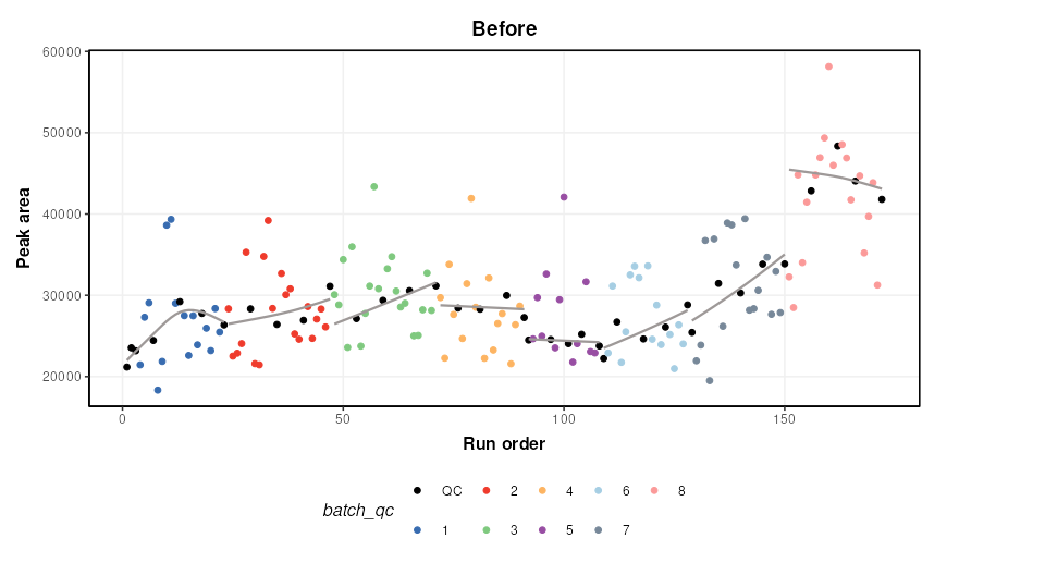

chart_plot(C,predicted(M))+ylab('Peak area')+ggtitle('After')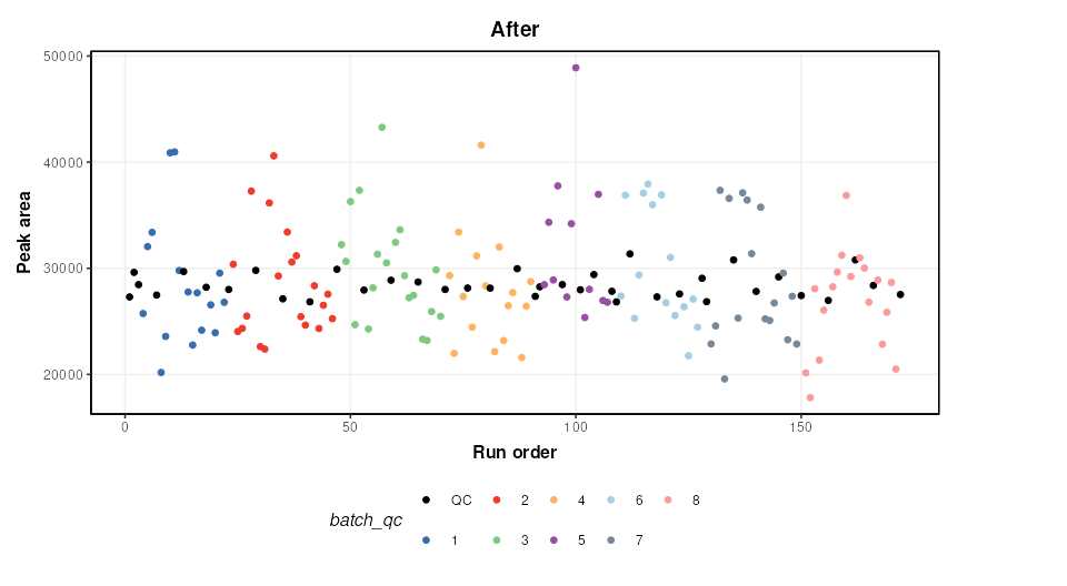

An additional step is added to the published workflow to remove any feature not corrected by QCRCMS. This can occur if there are not enough measured QC values within a batch. QCRMS in the pmp package currently returns NA for all samples in the feature where this occurs. Features where this occurs will be excluded.

M2 = filter_na_count(
      threshold=3,
      factor_name='Batch'
    )
M2 = model_apply(M2,predicted(M))

# calculate number of features removed
nc = ncol(DE) - ncol(predicted(M2))

cat(paste0('Number of features removed: ', nc))

## Number of features removed: 425

The output of this step is the output of MTBLS79_DatasetExperiment(filtered=FALSE).

Feature filtering

In the journal article three spectral cleaning steps are applied. In the first filter a Kruskal-Wallis test is used to identify features not reliably detected in the QC samples (p < 0.0001) of all batches. We follow the same parameters as the original article and do not use multiple test correction (mtc = 'none').

M3 = kw_rank_sum(
      alpha=0.0001,
      mtc='none',
      factor_names='Batch',
      predicted='significant'
    ) +
    filter_by_name(
      mode='exclude',
      dimension = 'variable',
      seq_in = 'names', 
      names='seq_fcn', # this is a placeholder and will be replaced by seq_fcn
      seq_fcn=function(x){return(x[,1])}
    )
M3 = model_apply(M3, predicted(M2))

nc = ncol(predicted(M2)) - ncol(predicted(M3))
cat(paste0('Number of features removed: ', nc))

## Number of features removed: 262

To make use of univariate tests such as kw_rank_sum as a filter some advanced features of struct are needed. Slots predicted, and seq_in are used to ensure the correct output of the univariate test is connected to the correct input of a feature filter using filter_by_name. Another slot seq_fcn is used to extract the relevant column of the predicted output so that it is compatible with the seq_in input. A placeholder is used for the “names” parameter (names = 'place_holder') as this input will be replaced by the output from seq_fcn.

The second filter is a Wilcoxon Signed-Rank test. It is used to identify features that are not representative of the average of the biological samples (p < 1e-14). Again we make use of seq_in and seq_fcn.

M4 = wilcox_test(
      alpha=1e-14,
      factor_names='Type', 
      mtc='none', 
      predicted = 'significant'
    ) +
    filter_by_name(
      mode='exclude',
      dimension='variable',
      seq_in='names', 
      names='place_holder',
      seq_fcn=function(x){return(x$significant)}
    )
M4 = model_apply(M4, predicted(M3))

nc = ncol(predicted(M3)) - ncol(predicted(M4))
cat(paste0('Number of features removed: ', nc))

## Number of features removed: 169

Finally, an RSD filter is used to remove features with high analytical variation (QC RSD > 20 removed)

M5 = rsd_filter(
     rsd_threshold=20,
     factor_name='Type'
)
M5 = model_apply(M5,predicted(M4))

nc = ncol(predicted(M4)) - ncol(predicted(M5))
cat(paste0('Number of features removed: ', nc))

## Number of features removed: 53

The output of this filter is the output of MTBLS79_DatasetExperiment(filtered=TRUE).

Normalisation, missing value imputation and scaling

We will apply a number of common pre-processing steps to the filtered peak matrix that are identical to steps applied in are described in Kirwan et al. 2013, 2014.

Probabilistic Quotient Normalisation (PQN)
k-nearest neighbours imputation (k = 5)
Generalised log transform (glog)

These steps prepare the data for multivariate analysis by accounting for sample concentration differences, imputing missing values and scaling the data.

# peak matrix processing
M6 = pqn_norm(qc_label='QC',factor_name='Type') + 
     knn_impute(neighbours=5) +
     glog_transform(qc_label='QC',factor_name='Type')
M6 = model_apply(M6,predicted(M5))

Exploratory Analysis

Principal Component Analysis (PCA) can be used to visualise high-dimensional data. It is an unsupervised method that maximises variance in a reduced number of latent variables, or principal components.

# PCA
M7  = mean_centre() + PCA(number_components = 2)

# apply model sequence to data
M7 = model_apply(M7,predicted(M6))

# plot pca scores
C = pca_scores_plot(factor_name=c('Sample_Rep','Class'),ellipse='none')
chart_plot(C,M7[2]) + coord_fixed() +guides(colour=FALSE)

## Warning: The `<scale>` argument of `guides()` cannot be `FALSE`. Use "none" instead as
## of ggplot2 3.3.4.
## This warning is displayed once per session.
## Call `lifecycle::last_lifecycle_warnings()` to see where this warning was
## generated.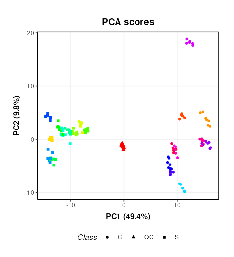

This plot is very similar to Figure 3b of the original publication link. Sample replicates are represented by colours and samples groups (C = cow and S = Sheep) by different shapes.

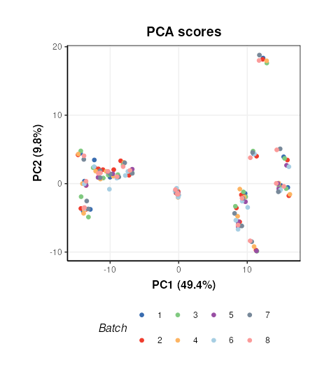
Plotting the scores and colouring by Batch indicates that the signal/batch correction was effective as all batches are overlapping.

# chart object
C = pca_scores_plot(factor_name=c('Batch'),ellipse='none')
# plot
chart_plot(C,M7[2]) + coord_fixed()